Chapter 6
Basics of Animation
In this chapter, you’ll set aside your rig briefly to take a general look at how animation happens in Blender. I’ll be introducing a few terms that anybody familiar with CG animation will know and presenting them in the context of Blender’s animation system. If you are new to CG animation, you’ll want to pay close attention because although the details are Blender-specific, the ideas are universal, and the functionality is essentially the same as you will find in any other 3D software.
- Keyframes and Function Curves
- Using the Graph Editor: Bouncing a Ball
- Interpolation and Extrapolation
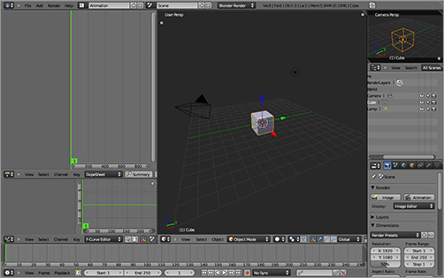
). This window does not require much vertical screen space, so in the default screen setup it runs along beneath the 3D viewport. You can also select the Animation screen configuration from the screen drop-down menu in the Information window header  (or by holding Ctrl and pressing the right or left arrow key to cycle through the configurations), which organizes your windows as shown in . This screen configuration contains most of what you need already laid out.
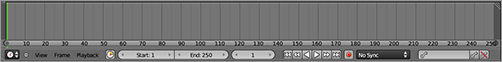
The Timeline
Default Animation screen
HOTKEY: Pressing Ctrl+right arrow or Ctrl+left arrow cycles through desktop configuration possibilities.
The Timeline’s basic functionality is self-explanatory. When you press the Play button  , the animation plays from the Start frame to the End frame on continuous repeat. The current frame is displayed in the field to the right of the Start and End fields, and you can input a desired frame number here directly. You can also use the left and right arrow keys on your keyboard to advance forward and backward by single frames, and you can use the up and down arrow keys to advance forward and backward by 10 frames at a time. Holding Shift and pressing the left or right arrow key will set the current frame to the start and end frame values, respectively.
HOTKEY: Pressing Shift+right arrow or Shift+left arrow sets the current frame to the Timeline Start and End frame values, respectively.
In addition to the play button in the Timeline, you can also play back animation by pressing Alt+A. Pressing Alt+Shift+A plays back the animation backward.
HOTKEY: Pressing Alt+A key plays the animation.
HOTKEY: Pressing Shift+Alt+A key plays the animation backward.
You’ll also want to look at a Graph Editor, so open a Graph Editor in one of the windows on your desktop. If you have selected the Animation screen layout, your Graph Editor will be displayed to the left of the 3D window, beneath the DopeSheet window.
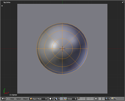
shows the sphere and the plane viewed from top view (7 on the numeric keypad).
Adding a plane and a ball
Move to front view (1 on the numeric keypad). Make sure the plane object is lined up with zero on the z-axis. Move the sphere to 10 Blender units (BUs) above zero along the z-axis.
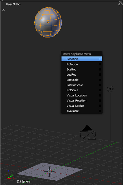
The first thing you’ll do is key the ball’s vertical motion. In Blender, you use the I key to insert a key. You want to key the ball at frame 1 at the high point of its bounce. On the Timeline, make sure you are in frame 1 (this is also displayed in the lower left of the 3D viewport). With the mouse over the 3D viewport, press I to insert a key, and choose Location, as shown in . You’ll see some horizontal lines appear in the Graph Editor, which represent the x, y, and z coordinates of the ball. You may need to scale the Graph Editor view using the Home key on your keyboard or using the scroll wheel of your mouse to see things clearly. The x and y coordinates are both 0, so these two lines lie on top of each other at the zero point.
HOTKEY: Pressing I inserts an animation keyframe.
HOTKEY: Pressing Home scales a view so that its contents are all fully visible.
Keying the ball’s location
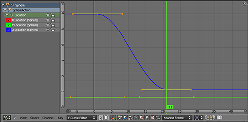
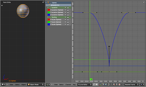
As in the Timeline, you can move back and forth one frame at a time in the Graph Editor using the left and right arrow keys, and you can move 10 frames at a time using the up and down arrow keys. Press the up arrow key twice to move 20 frames forward. The default frames per second setting is 24 fps (this setting can be changed in the Playback menu of the Timeline), so moving 20 frames forward moves you just less than a second forward in time. This is about right for the amount of time it will take for the ball to hit the ground, so move the ball down along the z-axis until it is touching the ground you created. Key this position in the same way you keyed the previous one. Note the curve shown in the Graph Editor in . The Z Location curve displayed in blue now dips from 10 to about 1.
Graph Editor
You have now added F-Curves to three channels, which are listed down the left-side shelf of the Graph Editor. The channels that are available for F-Curve creation depend upon the object selected and channels selected in this list. You can select or deselect objects and channels and make different channels visible or invisible using the eye icons next to the channel names.
Working with Control Points
By default, F-Curves are created as Bezier curves, with control point triples that enable you to adjust the shape of the curves manually. You can select control points by right-clicking the control point or using the B key’s Box Select tool to select multiple control points. You can select all the control points that share a frame by holding Alt and right-clicking. The A key toggles selecting all points and deselecting all points.
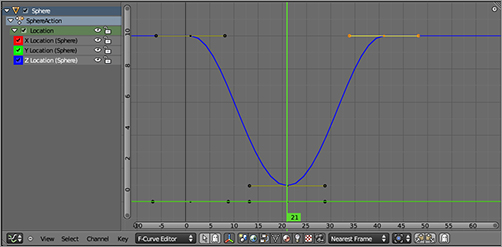
To complete the down and up bounce movement for the bouncing ball animation, select the first control point on the Z Location curve, representing the high point of the ball’s location. Duplicate this control point by pressing Shift+D, and move the copied control point to frame 41, as shown in . Hold the Ctrl key while moving the control point to constrain it to frames. You can also constrain the direction you move the keys to an axis in the window by pressing the X or Y key.
HOTKEY: Shift+D duplicates keyframes or key points on an F-Curve.
You now have a single up-down motion for the ball, which ends in the same place it begins. You can make a cycle out of it by setting the Start and End frames on the Timeline to 1 and 40. Note that the duplicate of the first key is actually at frame 41, so frames 1 and 41 are identical. This means that cycling from 1 to 40 gives you unbroken repetitions of up and down movement.
The full down and up cycle
Press Play on the Timeline to watch the ball move. You should see the ball rise and fall in smooth repetitions. (If there is any jerking movement, you need to check your keys and make sure they are the right values and placed correctly.) However, the motion is clearly not the motion of a bouncing ball. Bouncing balls do not drift smoothly up and down like this. You need to adjust the motion between keyframes. To do this, you need to edit the curves themselves.
Edit Mode
In the Graph Editor, you can edit curves that are in Bezier Interpolation mode as Bezier curves, using control points with handles you can manipulate. Selecting the center point of the control point enables you to move the entire control point, handles and all. Selecting either of the handles enables you to control the shape of the curve. With a control point selected, you can change the handle type under the Set Keyframe Handle Type menu, accessed with the V key. The options for handle type are as follows:
HOTKEY: Pressing V in the Graph Editor opens a menu to change the control point handle type.
Auto Blender automatically calculates the length and direction of the handles to create the smoothest curve.
Auto Clamped This is the same as Auto, except that control points at extremes of the curve are clamped horizontally. With Auto Clamped, local maximum or minimum points on the curve always run through at least one control point. This is the default.
Aligned Blender maintains a straight line between the two handles, so if you move one handle, the other one is also moved.
Free Either handle’s endpoint can be moved independently of the other handle.
Vector Both handles are adjusted to point directly to the previous and next control points.
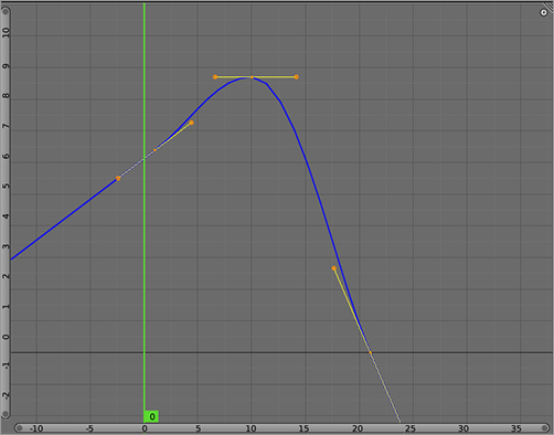
The main problem with the bounce curve is that the low point of the bounce is slowing down gradually and then speeding up when the ball returns upward. In a real fall, the object would continue to accelerate because of the force of gravity, so the curve would get steeper and steeper on the way down, before the ball is suddenly stopped by the unyielding ground. The ball retains most of its kinetic energy after this collision, but its direction is reversed back upward, which means it starts back upward with almost the same velocity it had when it struck the ground.
For this example, you’ll ignore the loss of energy and assume that the ball can keep bouncing forever, in which case the kinetic energy going upward out of the bounce is the same as that coming into the bounce. This energy, in countering the resistance of gravity, diminishes until the top of the cycle, when once again gravity takes over as the strongest force acting on the ball, and the ball comes down again.
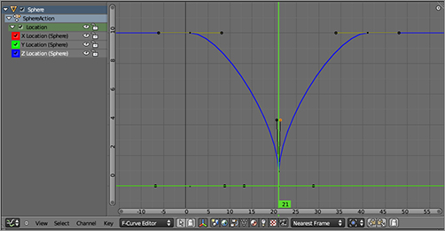
In practice, this all means you want two parabolic curves angling downward to meet at a point. You need to adjust the lowest point on the Z Location curve. Select the control point by clicking the midpoint of the control point triple.
A quick way to create a sharp vertex is to use the V key and select the vector handle type to change the handle type to vectors. Try this, and you will see that the handles now point in the direction of the preceding and following control points. This is an improvement, as you can see if you run the animation now. But the curves straighten out too soon, and the acceleration of the ball is not maintained all the way down. To adjust this, you can bring these handles’ controls closer together, making for a steeper curve. Editing a vector-type handle automatically changes it to a free type, so you can go ahead and select one of the handle points and press the G key, or you can right-click and drag the control point to move it slightly toward the middle of the curve, as shown in . Play your animation and see the improvement in the bouncing motion.
Sharpening the F-Curve at the bounce
Keying Scale: A Simple Squash/Stretch Effect
Now that the ball’s bouncing motion looks more or less right, you’ll add a little squash and stretch to add some more dynamism to the motion. The use of squash and stretch effects in this way dates back to early drawn animation, and the style at that time was inevitably cartoony.
Squash and stretch are real physical phenomena, but the exaggerated degree to which they are often used in animation is not realistic. Real squash and stretch depends upon the material of the object and the forces to which it is subjected. A steel ball and a water balloon, obviously, have different degrees of squash when bounced against a surface and different degrees of stretch when dropped from a height. Something like a baseball, for example, would have an imperceptibly slight squash and stretch in real life. Anyone who has seen photographs of a baseball contacting a bat knows that although the bat makes a deep instantaneous impression on the ball, the impression is quite local and does not alter the roundness of the ball very much. However, in a cartoon-styled animation, the squash and stretch for a baseball would be highly exaggerated to emphasize the dynamism of the ball.
You will take a very simple (and not very flexible) approach to animating squash and stretch here, simply keying values for scale. To do this, follow these steps:
1. Go to frame 1. With the ball selected in the 3D viewport, press I and select Scale. You should see keys appear in the Graph Editor and their corresponding channels appear in the list in the Graph Editor shelf, as in . If the channels are collapsed, you can click the gray triangle to get the view shown in the figure.
The original scale
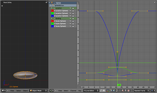
2. Select this first frame’s control points by holding Alt and right-clicking a control point in the first frame. Duplicate these control points with Shift+D. Move the new keys 40 frames to the right, holding down the Ctrl key.
3. Skip forward 20 frames (press the up arrow key twice) to frame 21, and scale the ball to a squash shape. To do this, scale the ball down along the z-axis to .5. Then scale again; this time, use S followed by Shift+Z to scale up in the other two directions to 1.5. Be sure not to change frames without keying this new scaling, or you will lose it (it will go back to whatever is keyed for the frame you go to; in this case, the first keyed value). Key the new scaling, as shown in .
HOTKEY: Pressing Shift+Z following a G, R, or S key transformation constrains the transformation to the plane defined by the x- and y-axes. Shift+Y and Shift+X behave similarly.
4. Because the ball is now scaled down vertically, you need to lower the low point on the Z Location curve so that the ball comes in contact with the ground instead of bouncing back just short of it. Do this by selecting the center control point on the Z Location F-Curve and lowering it with the G key and the down arrow button on your keyboard. Adjust it until your squashed ball is properly set on the ground. You do this by editing the curves directly; if you simply moved the ball onto the ground in the 3D view and then reset the key with I, you might lose your special edits to the handles of the F-Curve at that key.
5. The stretch effect is a result of gravity and should be at its maximal point at the same time that the gravitational acceleration is highest. This is, of course, the frame immediately before the ball makes contact with the ground. Go to this frame and press Alt+S on the ball to clear all scaling. Then scale up along the z-axis to 1.25, and scale down along the x,y plane to .75. Key the scaling.
Scaled to a squash shape
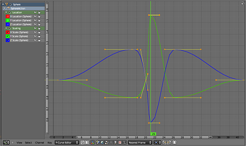
6. Because the kinetic energy of the ball is still high on the recoil, it should spring back into the stretched position quickly, but because it is not influenced by hitting a solid surface, it does not have to spring back within the space of a single frame. Duplicate the stretched key from frame 20 and place it a few frames after the actual contact frame. The squash scaling also should not begin early. The ball should squash on impact. shows the final key frame positions for the stretch scaling.
Placing the stretch keys
.
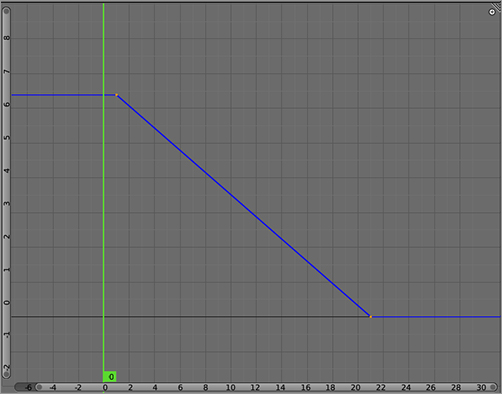
Bezier interpolation
This curve type creates the most naturalistic movement of the three types, although this does not mean that unadjusted Bezier curves will always produce convincing movement. It is important to consider the physical forces being applied to the object, as discussed in the previous section.
An equally important quality of Bezier interpolation is that it is the only interpolation type that allows editing of the shape of the curve itself.
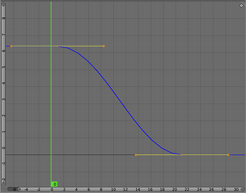
Linear Interpolation
Linear interpolation creates a straight line between keyed values. This can be useful for mechanical movements, but it is also useful for animating properties other than movement, which might change in a linear fashion. Linear interpolation is not a convincing way to model organic movement. Editing the shape of the curve is also highly restricted. In the Graph Editor, you can move key points around freely, but you cannot change anything else about the shape of the curve. shows a linear interpolation between points.
Linear interpolation
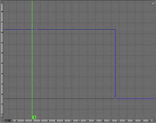
Constant Interpolation
Constant interpolation holds each keyed value constant until the next value is keyed, as in . This does not model motion at all but rather sudden, discrete changes in position or value. This is the interpolation mode to use for instantaneous changes. In fact, when keying an object’s layer, this is the only interpolation mode possible. For animation, the constant interpolation mode might seem useless to novices, but it can be very effective at blocking out the key poses of an animation sequence, making sure the gross timing is correct before going on to further refine the animation.
Constant interpolation
Extrapolation Types
There are two extrapolation types: constant and linear. You can use these types with any of the interpolation types. In the following examples, they are shown with a curve using Bezier interpolation. I have included two examples for each—one with two key values and one with three—to emphasize cases in which this makes a difference to the behavior of the curve. You can access these in the Extrapolation mode submenu of the Key menu.
Constant Extrapolation
Constant extrapolation holds the values of the first and last keyed values constant in the positive and negative directions on the Timeline. shows constant extended curves in cases with one and two key points. Constant is the default extend value.
Constant extrapolation with two and three key points
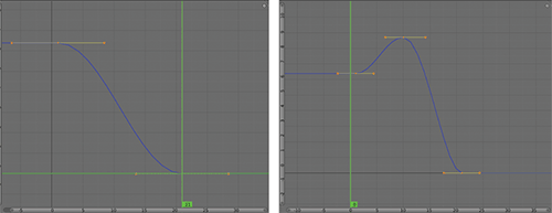
Linear Extrapolation
Whereas the constant extrapolation type holds the value constant, linear extrapolation holds the angle at which the curve passes through the first and last keyframes constant and calculates the continuation of the curve as an extension of the line at that angle, as shown in . You can use two points to create a straight F-Curve at any angle. You can use linear extrapoloation, for example, to continue certain transforms indefinitely, such as rotation. A linear extrapolated curve with two defining values on the rotation curve is a good way to animate a spinning wheel.
In the case of three or more points, the extrapolation extend appears as in . This is a much less common use of linear extrapolation.
Linear extrapolation with two key points
Linear extrapolation with three key points
F-Curves and F-Curve Modifiers
F-Curves are the basis of all animation in Blender. Any time a value changes, there is an F-Curve guiding its change. In the next few chapters, you will see a number of different ways and places in which you can create and manipulate keys; you can key some values in the Properties window by pressing the I key over a field, you can key some values by using sliders, and much of the armature-based work you will be doing will take place in the DopeSheet window and the Non-Linear Animation Editor. Nevertheless, all these contexts are fundamentally interfaces laid over the basis of F-Curves and key point values. It is important to remember that when problems arise in these other areas, you can always find the F-Curve that’s giving you trouble in the Graph Editor and find out what’s going on with it directly.
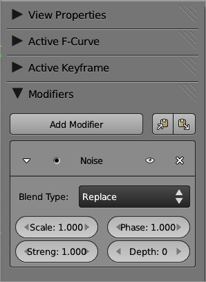
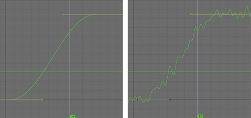
F-Curves can also be nondestructively modified by using F-Curve modifiers. You can access F-Curve modifiers in the Properties Shelf of the Graph Editor window with an F-Curve selected and editable. A variety of types of modifiers enable you to change the shape of the curve in many ways. shows a Noise-type F-Curve modifier that adds a random component to the curve. shows a simple F-Curve before and after the modifier is activated. Like Object modifiers, F-Curve modifiers can be deleted or deactivated.
Noise F-Curve modifier
Noise-modified F-Curve
You can use modifiers to create cycles, steps, or limits in your F-Curves, apply built-in functions to the curves, and even influence the F-Curve values using Python, giving you a huge amount of power over the shape of the curves.
In the next chapter, you’ll step away from this low-level F-Curve view of animation and look at practical tools for animating fully rigged characters.

