Chapter 7: Vector Nodes (V)
Vector nodes transform XYZ information. Of course in a 3D application there is a lot of different vector information. The vectors of the most interest are texture coordinates and normal maps. As you can see from normal maps, color information can be transformed into XYZ and back. So the line between vector and color node is fluent. As you can see from the coordinate system in Blender, X is represented by red, Y by green and Z by blue. However rotating vectors is a lot easier than remembering how to alter the RGB so the rotation will match, so for vector transformations, the following nodes are quite handy.
Mapping (M)
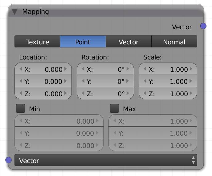
This node is able to read texture input coordinates and transform them. One of the first uses that comes to mind for conventional texturing is using the scale to map a seamless image onto your surface without having to scale the UVs to a ridiculous size. But it can also be used to rotate or offset your textures. This is even more important when you are using 3D textures. All procedural textures are three dimensional. This way they will map seamlessly onto every surface, but if you use UV coordinates for the input you will end up with seems. So those textures will be usually used with generated coordinates, which you have very little control over, until you insert this node.
Leaving the vector input on a texture blank will make Cycles choose what input to use based on the type of texture, but the mapping node needs a vector plugged into the vector input.
To make the node more intuitive, you can choose the way the transformations will happen, more precisely: the order.
Location
Moves (translates) your texture along the X, Y or Z axis.
Rotation
This offset will rotate the texture around the X, Y or Z axis.
This operation is the same for all four modes.
Scale
Use this value to stretch your texture along the X, Y or Z axis.
Min
You can set a minimum value, which means every point of your texture that would theoretically be projected before the minimum coordinate will get clipped. This results in a stretch of the pixels at the border across the clipped area, so ideally they should be unicolored, to avoid banding .
Clipping will be calculated before an optional rotation.
Max
You can set a maximum value, which means every point of your texture that would theoretically be projected after the maximum coordinate will get clipped. This results in a stretch of the pixels at the border across the clipped area , so ideally they should be 100% transparent.
Clipping will be calculated before an optional rotation.
Hint: Min and Max can be used to clamp decals, so they do not get repeated all over your object.
Modes
Texture
In this mode Cycles will use the inverse of the values you enter. This can be more intuitive, because some may find it a little strange when an increase in scale shrinks your texture.
If so, you will probably like this mode best. This also means that if you move your texture in positive x, in this mode it will actually slide to the right just as you might feel it should.
Additionally its location values are relative to your texture, not the scale of your object, so an offset of 1 in either location will not visibly affect the displayed texture, because it was offset by 100% its size and gets repeated to exactly where it was, 0.5 will offset it exactly half the size of your image.
Point
In this mode the transformations are applied as a mathematician would expect. If you, for example, increase the scale to 2, 2, 2, your texture will appear half as big, because effectively it’s canvas got enlarged with the texture keeping its size. Then the canvas got mapped onto the same size surface, making the texture look smaller on said surface. Also if you move coordinates to the right – you may know this from the UV editor – the texture will slide to the left, because effectively the surface slides to right, while the texture stays in the same place.
Vector
In this mode the location values will not change anything.
Normal
Outputs a normalized vector, this is not to be confused with the normal vector of a face. It is called normal because it is a unit vector and therefore has the normalized length of 1. In this mode location will not make a difference. Using a unit vector only produces useful result if you use it with certain coordinate inputs. For example if you use it with the option, your texture will be projected onto your object, starting at the origin. On the adjacent faces the texture will be stretched, but on the opposite faces the texture will appear as if they were a screen the projector shines onto. If you use as an input, the texture will behave similar to the reflection input, but zooming in or out on your object will not scale the texture.
Vector (input)
Coordinates, usually coming from an input node.
Vector (output)
The transformed vector.
Bump (B)
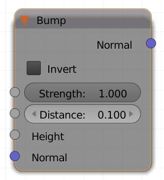
If you don't have a proper normal map, but still want to use a different bump for individual shaders you can use the bump node. It also has more options than the displacement input of the material output node.
A bump map is usually a black and white image, where white areas will appear to stand out from the surface and black areas will look as if they were chiseled into the surface. This way it simulates distortion the surface of a shader, without having to increase the polycount. For more information about adding detail to surfaces without increasing the polycount, see below.
For more details on the difference between bump and normal maps, see .
Invert
White now pushes down areas and black makes them stand out.
Strength
A multiplier for the effect of the bump map.
Distance
Multiplies this value by the height input. Increasing the value will make the bumpmap act as if the object was further away, therefore the absolute depth of the groves would be bigger. It drastically darkens the areas that are being pushed down.
Height
Input for the bump map to be used.
Normal (input)
You can combine a bump map with a normal map, by using the normal out of the normal map node with the normal input of the bump node. It is fairly complicated to mix normal maps, however a good approximation can be achieved by using a bump node with the output of a normal map as the normal input.
Normal (output)
Returns a normal map to be used with the normal input of a shader node.
Normal Map (N)
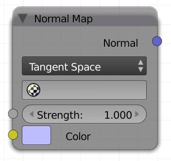
You can tell an image is a normal map when it mostly contains light blue and magenta colors, but also green and brown can occur. In short a normal map simulates bumps and dents in your object without increasing the polycount.
To use a in Cycles, you need one of the aforementioned images as an input. In the image texture node, be sure to set the color space to non-color data.
It receives a color and outputs a vector. This is mathematically correct, since its RGB represent X, Y and Z transformations, but you should probably not use this vector as an input for mapping, the correct use is connecting it to the normal input vector of a shader or Fresnel node.
You can easily select the UV map to use for this texture, without having to use an attributes or UV map node.
You can change the strength of the normal map, increasing this value will result in a more displaced looking surface. It is good practice though to create your normal map again, with different values if you are not happy with the results. But usually you will get away with just altering the strength.
For more details on the difference between bump and normal maps, see .
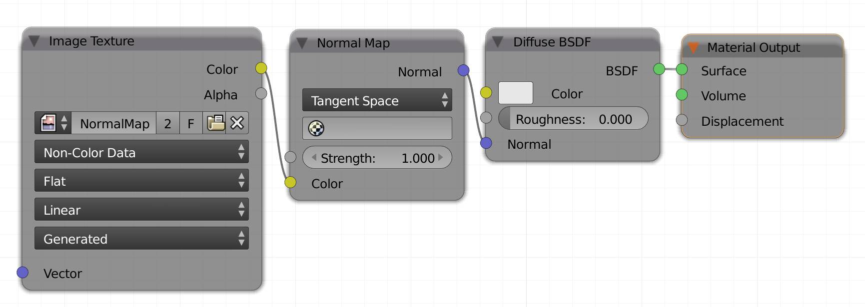
Fig. 7.1) The correct way to use a normal map in tangent space, note that the image texture node is set to Non-Color Data. Leaving the field in the normal map node blank will make Cycles use the default UV map.
You can choose from several modes:
Tangent Space
This is the standard method. If you use external programs with very few exceptions they will create a normal map suitable for tangent space. Those are the typical blue/magenta and sometimes with some green and brown maps you find. The neutral color in this mode has the Hex Code 8080FF. Parts of the normal map that are of this color will not change the way light interacts with the surface.
There is a huge difference between the tangent normals and the rest. The tangent normals are used to displace a surface, the rest of them are supposed to be used as texture coordinates. You can bake the normals of a surface, while taking into account surface displacement. So the following modes offer you the possibility of using normal as input for a texture coordinate, which will then follow the dents and bumps of the surface.
Blender World Space
If you used Blender to bake the textures in world space, choose this option, since it is more suited this way.
Blender Object Space
If you used Blender to bake the textures in object space, choose this option, since it is more suited this way.
World Space
Use this option if you used a third party software you to bake the normal map with world space for export / bake settings.
Object Space
Use this option if you used a third party software you to bake the normal map with object space for export / bake settings.
Little textured sphere
You can quickly choose a UV map different from the standard map (the one with the camera turned on in the data UV Maps box) without using an additional attribute or UVmap input.
Strength
You can adjust the strength of the effect.
Color
Your normal map goes in here.
Vector
Outputs a vector that, if set to tangent, is used as an input for the normal vector input of most of the shader nodes. The other settings are more commonly used to have full control over the normal input for texture coordinates.
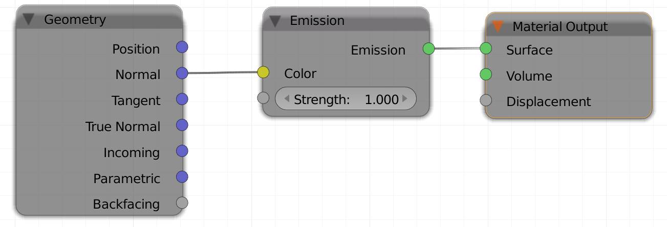
Fig. 7.2) the normals of an object can be visualized by plugging their vector information into the color input of a shader.
Normal (O)
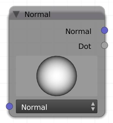
You can use this node either to generate a normal vector, or to calculate the dot product of an input vector.
Normal (in)
You can input a vector here, To get reasonable output use the normal vector from the texture coordinate node as input.
Normal (out)
This ignores the input as it generates a vector itself. It outputs one vector only, which will be used across the entire object. The direction of the normal vector can be chosen by dragging the big sphere in the node.
Dot
Calculates the of two vectors. If the two are orthogonal, the result will be 0, if they are antiparallel, meaning they point in opposite directions, the dot will be -1. The two vectors that are compared by this node are the normal of each face and the direction, which you can alter by clicking and dragging the sphere.
Essentially if you use the dot as a color for a material it will make your object seem as if it was illuminated from the local direction you choose with the sphere.
Note: These values will be normalized, so no output value higher than 1 is possible.
Hint: you can use this node to fake a specular , by using a color ramp to control the hardness. See fig. 7.3 below.
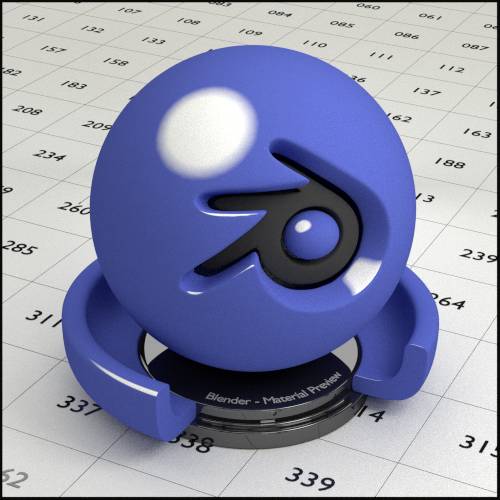
Fig. 7.3) Fake Specular using the normal texture coordinates, for the node setup see image below. This example used a diffuse material with a color ramp to control the color and size of the spec. In combination with a texture you can use a color mix node set to add.
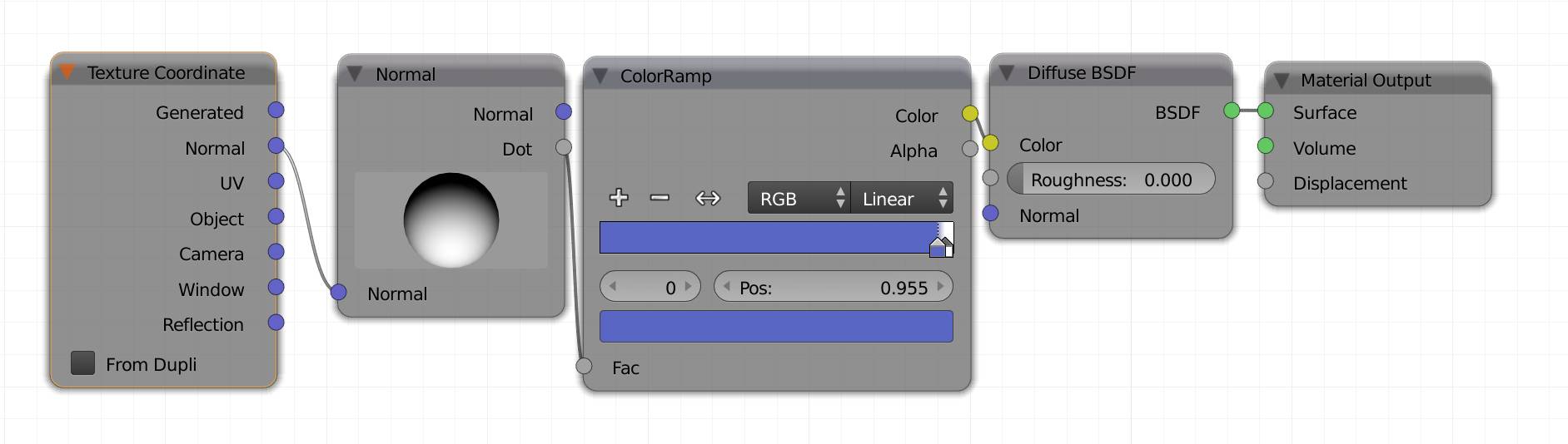
Fig. 7.4) Node setup for fake specular material. Using this setup you can control the position of the spot with the sphere of the normal node. The size can be adjusted with the color ramp node. This setup is popular for the gleam of an eye to make it look more alive.
Vector Curves (V)
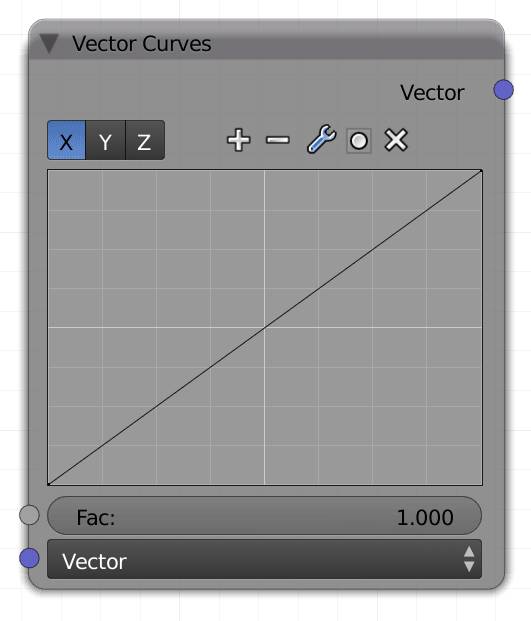
Just as you can adjust RGB values separately with the node, you can transform the X, Y and Z values separately. This way, you get a smoother transformation than by just adding values or multiplying them. Also you will be able to leave the start and the end of the vector untouched, while distorting everything in the middle.
So let’s say you take a plane and map an image across it. Then the local X position of the image will be represented in this node from left to right. If you then click in the middle of the curve and drag it upwards, the texture will be stretched towards the center of the face, keeping its boundaries (see fig. 7.5) Note that other than the RGB curves the lower left corner represents -1/-1 and not 0/0. This means you can also modify negative coordinates that you might get from object input or similar.
You can use the + and - buttons zoom the grid in and out to get even more precise control over your curves.
If you click on the wrench you can choose from these options:
Reset View
In case you zoomed in or out using the + or – symbol, this will undo those changes and set the zoom to its original value.
Vector Handle
The standard method of interpolating between two points is auto, somewhat similar to Beziér, vector handles will result in a linear interpolation.
Auto Handle
The standard method of interpolating between two points is auto, somewhat similar to Beziér, In case you set this to vector, you can use this function to reset it to auto.
Extend Horizontal
The two extend-options only affect the curve before the first and after the last point. For extend horizontal, the curve outside of the first and last point will be horizontal, meaning all points after the last point will get the same Y (transformed) value as the last one and vice versa for the first.
Extend Extrapolated
This is the standard setting, so it will only influence anything if you previously chose Extend Horizontal. This option only does any changes if you move the right- or leftmost point on a curve. If it is set to extrapolate, the curve beyond this point will continue with the incline of the last dot on the curve and vice versa for the beginning.
Reset Curve
Can be used to reset the curves, assigning all points the same Y value as their X value is and deleting all manually inserted dots for X, Y and Z.
Clipping Options
Using the little circle you can clip the area in which the dots can be moved, preventing you from moving them too far for your taste by accident.
Delete Points
If a dot is selected, you can delete it with the x symbol.
Fac
How strong the effect is. Typically you will leave this at one, if not the original image gets calculated back into the corrected one. It can be useful however to limit the effect to certain areas using a texture.
Vector
Input for the Vector to be transformed.
You can use this node to distort images. This can be particularly useful to distort procedural textures, so they are either less repetitive or more interesting.
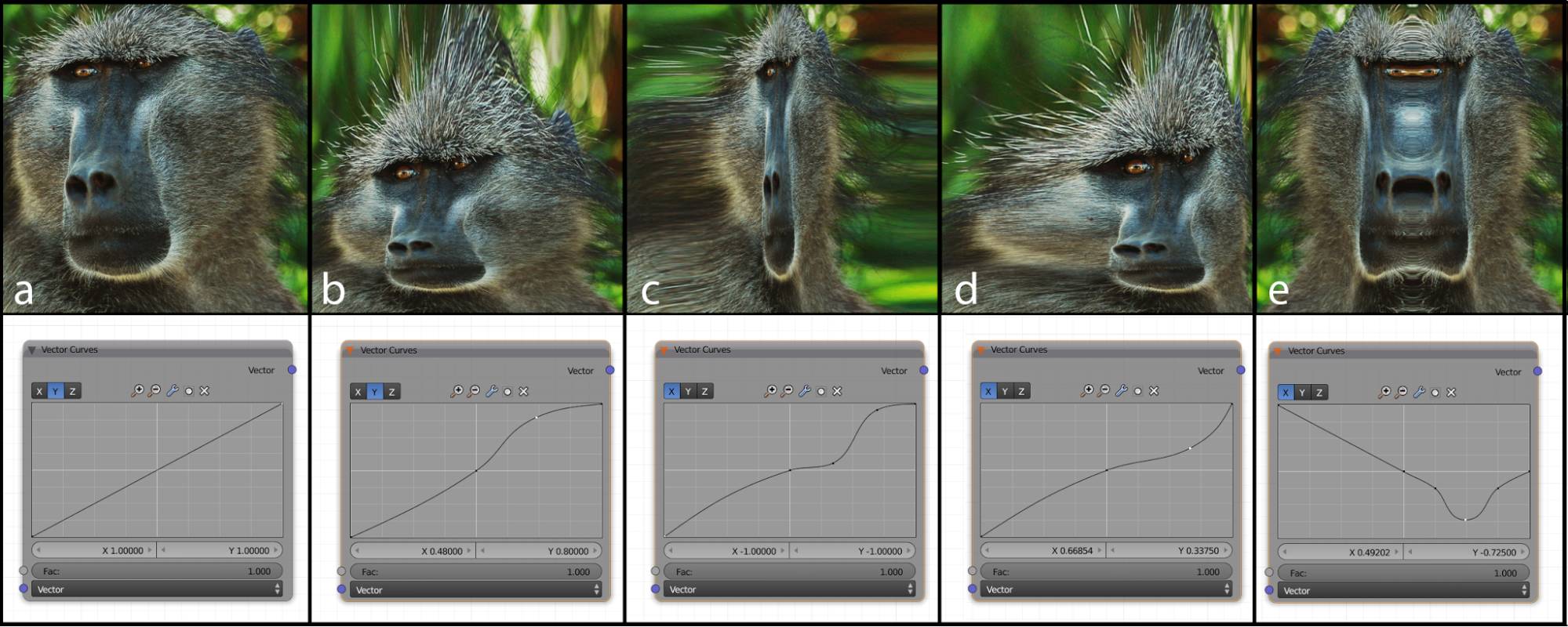
Fig. 7.5) An image texture distorted by the vector curves node. The according settings for the vector curves are displayed below the rendering. a) undistorted image, in d) the X and Y curves were modified in the same way. The values below and to the left of the center were ignored. This is because the generated input only uses positive x and y values. The point at 0,0 was move to 0,1, so the interpolation would not interfere with the part using transforming positive x values.
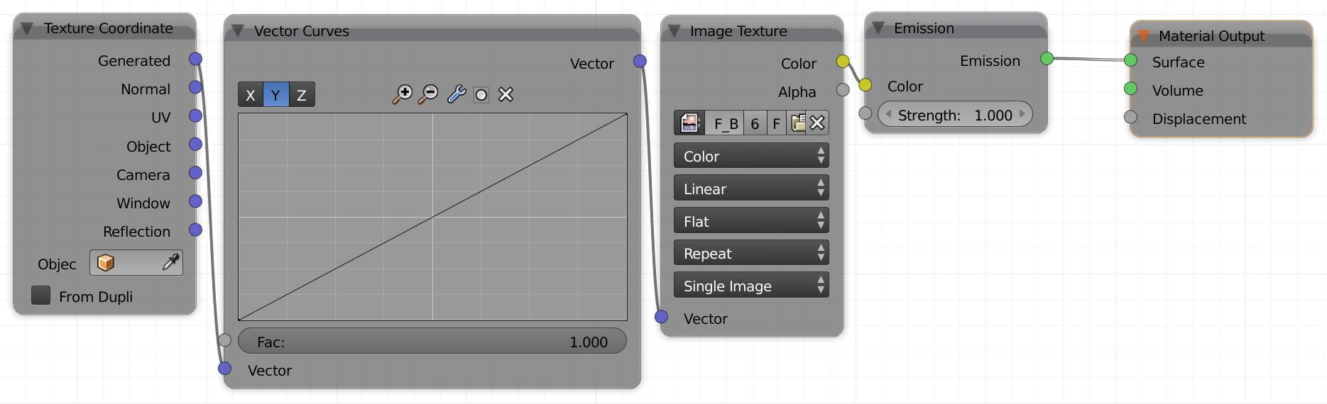
Fig. 7.6) Node setup for the rendering above.
In fig. 7.6 Vector curves were used to distort the positive x and / or y values of the texture coordinates. Raising the curve at either end stretches the image towards the other end and vice versa. In order to compensate for this the other half of the texture gets stretched. In e) the value for x = 0.25 and 0.75 were mapped to the same value. This resulted in a mirroring effect of the image.
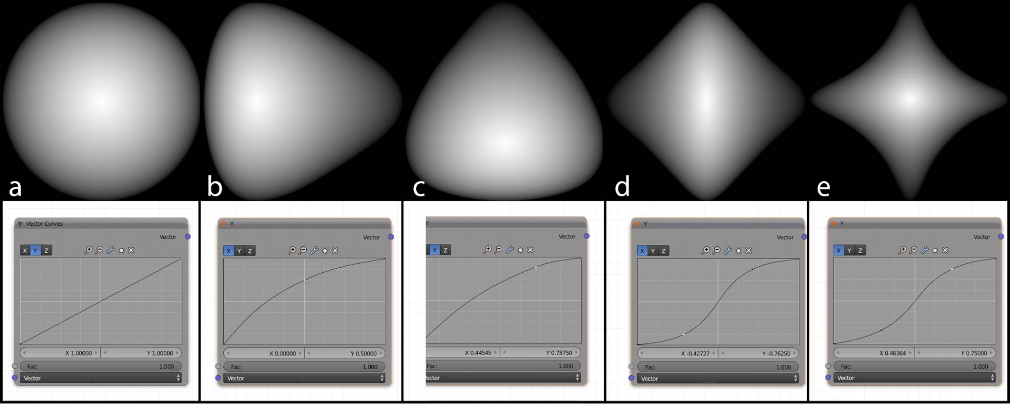
Fig. 7.7) A gradient texture set to spherical. The input used for the texture coordinates was object, which means the center (0, 0) was in the center of the object and it allows negative x and y values. This implies that the center of the circle was actually at 0,0 as well. Distorting the curves only on one side resulted in a pear shaped distortion. In d) both sides were squished, resulting in a diamond shape. In e) both x and y curves were manipulated the same way.
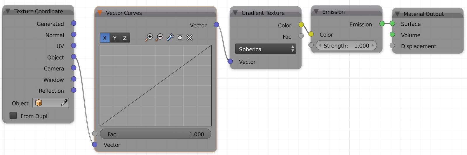
Fig. 7.8) Node setup for the rendering above.
In fig. 7.8 you can see a circle mapped onto a plane by using the object input coordinates. This means half a circle is drawn across from -1 to 1 in x and one half in y. It is important to note that thereby parts of the image were mapped onto negative coordinates that behave in the same way as positive, only in the opposite direction. The effect of curve manipulation were similar in fig. 7.5 and 7.7 but the object input used the entire spectrum of the vector curves as opposed to only the positive half.
Vector Transform (T)
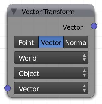
This node allows you, among other things, to use settings that work for one object in one orientation to work for all objects, regardless of orientation.
For example, you can create what’s called slope dependent materials. For this you would convert the normals of an object from object to world space. You can also transform the world or object space normals to camera space. You can - of course - use this node for more things than just that, but as a final example you can convert world to object space to create a gradient across objects regardless of their orientation.
You might know local position or scale from parenting relations in the viewport. For this node, though only the rotation vector is relevant. So in a way it will compare the input vector to the rotation of the object and match them.
Type
The outgoing vector can either be a point, a direction (vector) or a vector with a length of 1 (unit vector)
Convert From
The type of coordinate space convert from. This can be set to either world, object or camera.
Convert To
The type of coordinate space convert to. This can be set to either world, object or camera.
Vector (Input)
The vector you want to transform.
Vector (Output)
The transformed output vector.

