Chapter 6: Color Nodes (C)
The color nodes family will help you adjusting colors as well as brightness of textures or maps. They are very useful, since you don't have to go back into your image editing software to make little adjustments.
All color nodes have a factor which controls how strongly the effect is applied. It mixes the result of the node with the original image by the factor specified. This is most commonly used in combination with a grayscale map to limit the effect to certain areas of your surface.
MixRGB (M)
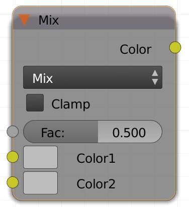
The color mix node offers a wide variety of what to do when you want to combine two images. There is a certain type of math behind each transfer or blend mode. I will state the math, but mainly focus on what the node does effectively in plain English.
The mix node comes with a factor, determining the strength of the effect. The upper color socket (Color1) determines the base color, the lower socket (Color2) the one mixed into it determined by the Factor. Of course you can also use a grayscale map to limit the effect to certain areas.
It also has a clamp checkbox, for example add mode can produce values greater than 1. Since the image is 32 bit until you save it in lesser color space, values greater than 1 will be allowed, but can produce unwanted results, especially on diffuse shaders. Cycles textures are essentially 32 bit per channel. Clamp will not let any pixel get brighter than 100% or darker than 0%.
Note: This node treats alpha as black.
I f you don't like math and never will, you can safely skip this paragraph and just look at the pretty pictures further down.
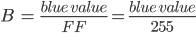
The node will split every pixel into its RGB values, do the transformation and then mix them again. Each pixel can be expressed by 6 digits in hexadecimal numbers. That means they don't have digits from 0 to 9 but from 0 to 15, the last 6 digits are represented by letters. FF is the highest number, it is 16 * 16 - 1 = 255, because we start counting at 0 so instead of 1 to 256 we have a range of 0 to 255. Just as the highest two digit number is 99, 10 * 10 - 1 = 99.
So the hex code works as follows:
FFFFFF is pure white, since it is the highest number you can reach with 6 spaces filled by digits from 0 to 16. This also means that the Blender color picker can distinguish between 16.8 million colors, 16 6 which is the depth of an 8 bit color space, where there are 2 8 variations for each color channel and 3 color channels resulting in  .
.
For the following examples, each pair of digits representing one color is normalized, then calculated separately and recombined in the end. To normalize a value, you need to divide it by the highest number possible in your range.
 ,
,  ,
, 
So you will get a number between 0 and 1 for each channel.
This is why I will only show the transformation once, using numbers between 0 and 1, since it repeated the same way for all three color channels. Let’s call the value input of the upper socket a , the one of the lower socket b . The reference for the output will be r for result.
Some color blend modes treat grayscale values differently than color values. I will refer to black, white and gray, where R = G = B and therefore the saturation is 0 as neutral colors .
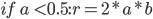
Since this chapter would be really boring for people not interested in math and it is fairly hard to imagine what a mathematical function does to two images, we rendered three images per mode, one a composited a over b, one flipped and a desaturated version.
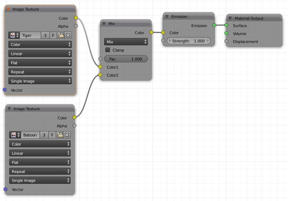
Fig. 6.1) Node setup for the Mix Node demo images. The blend type of the mix node was changed to the according type and the factor was always left at 1. For images 6.2 - 6.19 b) and c) the two input sockets of the mix node were flipped, so the baboon became Color1 and the tiger Color2.
Mix
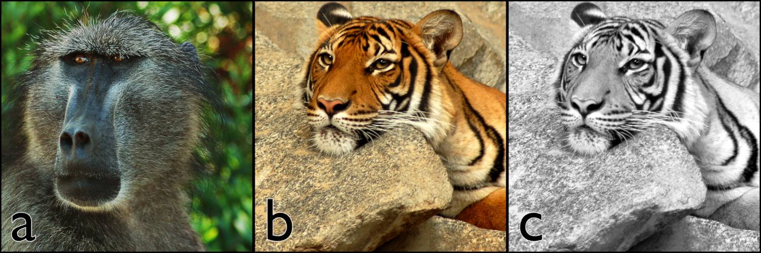
Fig. 6.2) In this version you can see the original images, since they were mixed by 100% leaving Color2, which was baboon in a), and tiger in b) and c). In c) the setup of b) was rendered, but both images were desaturated before mixing them. For the node setup see fig. 6.1.

Will output the mean value between the two color slots, mixing them by the factor specified.
Add
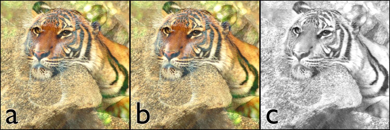
Fig. 6.3) 2 images mixed by the blend type add . For the original images compare fig. 6.2, For the node setup see fig. 6.1, in b) and c) the inputs for the mix node were switched, in c) the images were desaturated before getting mixed.

This brightens the image considerably. Adding white (1) will result in a white pixel, adding black (0) will not change the result. Since there is a chance for a value to be higher than 1 (0.6 + 0.5 = 1.1), there is an option to clamp values to the range from 0 to 1.
Multiply
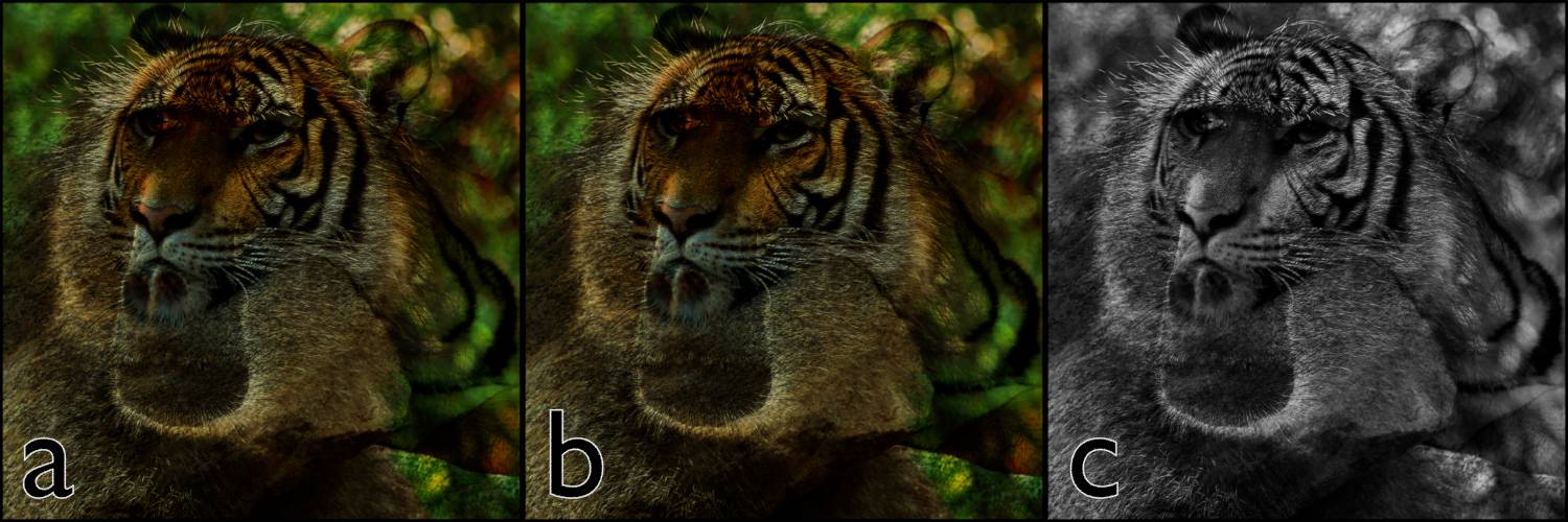
Fig. 6.4) 2 images mixed by the blend type multiply . For the original images compare fig. 6.2, For the node setup see fig. 6.1, in b) and c) the inputs for the mix node were switched, in c) the images were desaturated before getting mixed.

Since a) and b) are both smaller or equal to 1 in an 8 bit color space, this will darken your image. Anything multiplied by 0 (black) will result in black. Multiplying by 1 does not change your value, so pixels multiplied by white will stay the same.
Subtract

Fig. 6.5) 2 images mixed by the blend type subtract . For the original images compare fig. 6.2, For the node setup see fig. 6.1, in b) and c) the inputs for the mix node were switched, in c) the images were desaturated before getting mixed.

This of course darkens the image as well, but more drastically than multiply.
Screen
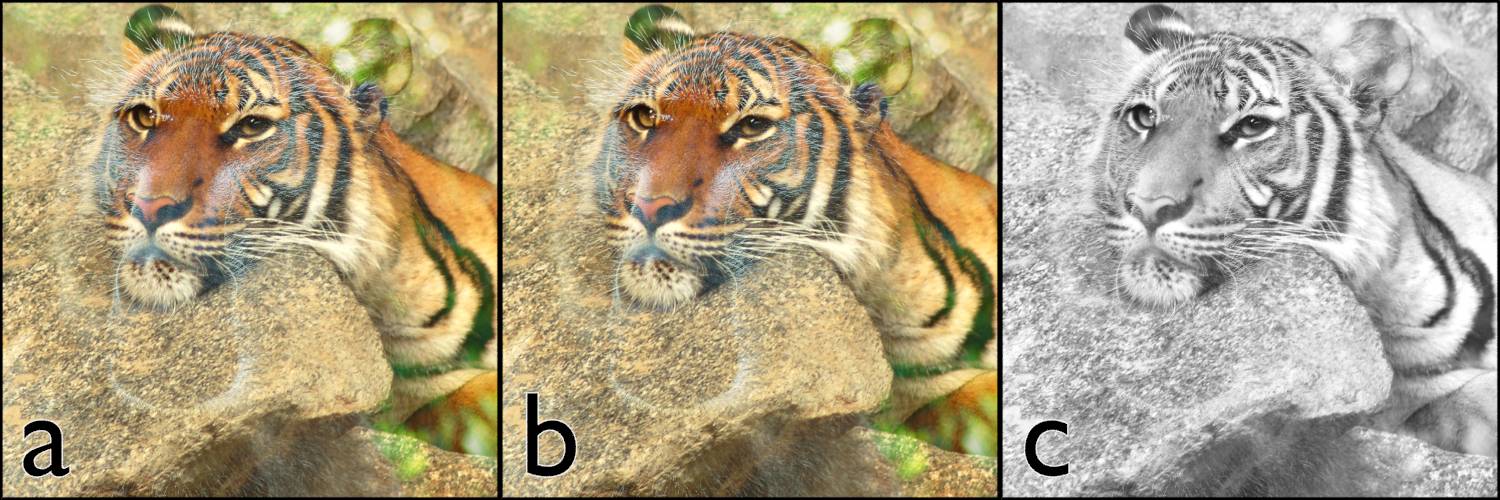
Fig. 6.6) 2 images mixed by the blend type screen . For the original images compare fig. 6.2, For the node setup see fig. 6.1, in b) and c) the inputs for the mix node were switched, in c) the images were desaturated before getting mixed.
This mode will brighten your image, but not as much as add will. The technical term is inverse multiplication, but it is called screen, because you can imagine two beamer s projecting two images on top of the same canvas. Since projecting black on top of any other color will not change anything, this applies for screen mode as well.
Divide
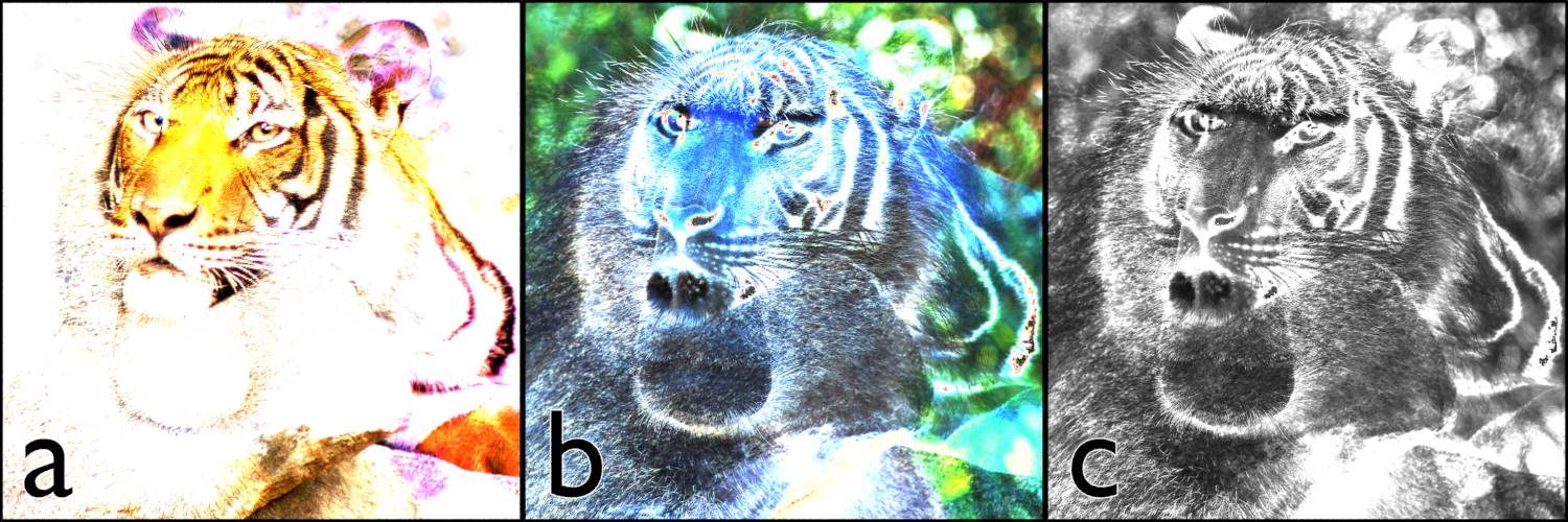
Fig. 6.7) 2 images mixed by the blend type divide . For the original images compare fig. 6.2, For the node setup see fig. 6.1, in b) and c) the inputs for the mix node were switched, in c) the images were desaturated before getting mixed.

Remember that we are dealing only with values between 0 and 1, dividing by 0.5 is the same thing as multiplying by 2, so divide actually brightens your image.
Division by zero will be treated like adding 1, resulting in a white pixel.
Difference
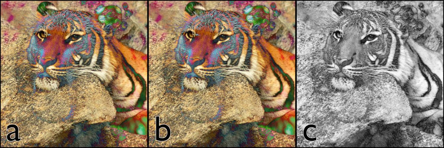
Fig. 6.8) 2 images mixed by the blend type difference . For the original images compare fig. 6.2, For the node setup see fig. 6.1, in b) and c) the inputs for the mix node were switched, in c) the images were desaturated before getting mixed.

Since a difference is always positive, Cycles will only take the absolute value of the calculation, there is no negative color value. If you desaturate the output of the difference node, you will get a map that shows the difference between two pixels by their resulting brightness.
Darken
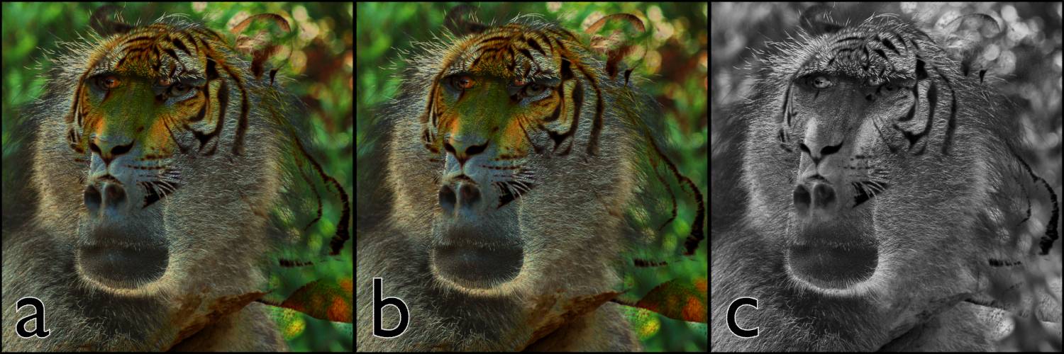
Fig. 6.9) 2 images mixed by the blend type darken . For the original images compare fig. 6.2, For the node setup see fig. 6.1, in b) and c) the inputs for the mix node were switched, in c) the images were desaturated before getting mixed.


This mode will compare two pixels and outputs the darker one of the two unchanged. This darkens the image, but in a very unnatural way.
Lighten
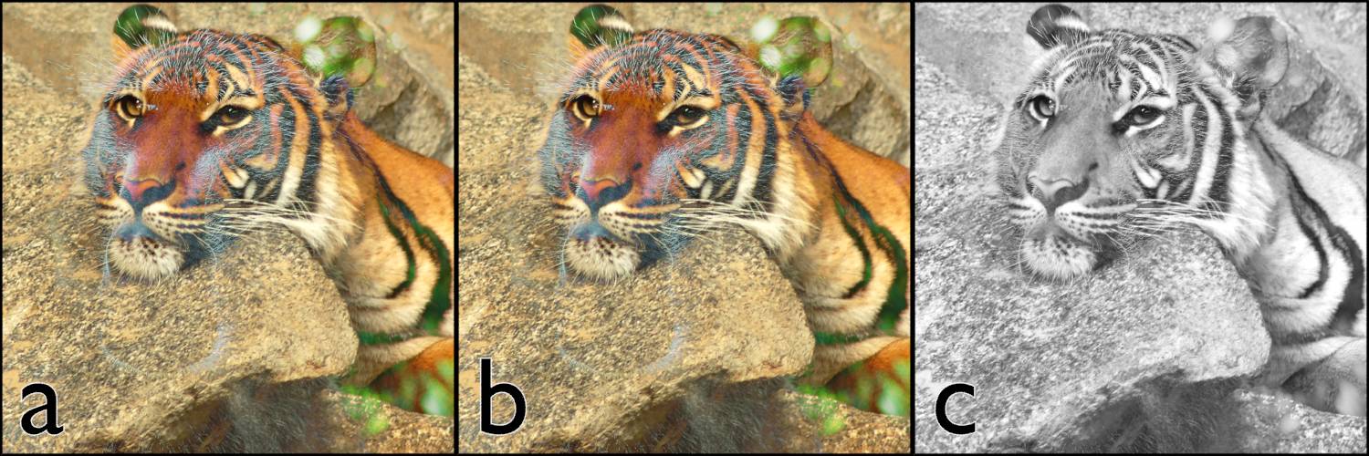
Fig. 6.10) 2 images mixed by the blend type lighten . For the original images compare fig. 6.2, For the node setup see fig. 6.1, in b) and c) the inputs for the mix node were switched, in c) the images were desaturated before getting mixed.


This is the opposite of darken. It will compare two pixels and output the brighter one of the two unchanged.
Overlay
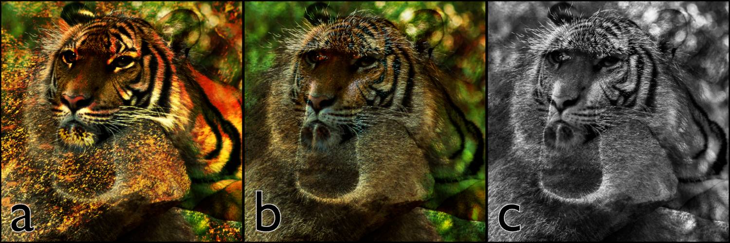
Fig. 6.11) 2 images mixed by the blend type overlay . For the original images compare fig. 6.2, For the node setup see fig. 6.1, in b) and c) the inputs for the mix node were switched, in c) the images were desaturated before getting mixed.
 (similar to multiply)
 (same as screen)
For some this may seem pretty intimidating, but let's just say overlay greatly enhances the contrast of your image, but darkening it overall. It is a combination of screen and multiply mode, depending on the color value (lightness).
Dodge
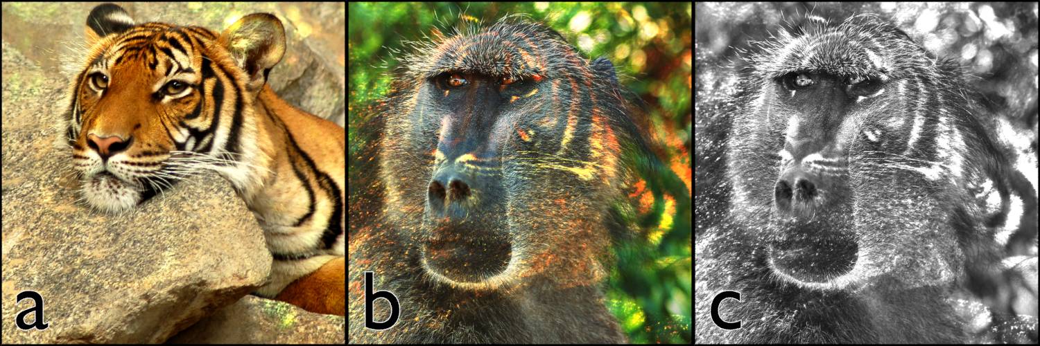
Fig. 6.12) 2 images mixed by the blend type dodge . For the original images compare fig. 6.2, For the node setup see fig. 6.1, in b) and c) the inputs for the mix node were switched, in c) the images were desaturated before getting mixed.

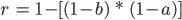
This can be seen as the inverse of the multiply mode, since the values get divided instead of multiplied. It will brighten your image as well as increasing the contrast. In case 1 - b is smaller or equal to 0, the return value is 1.0.
Burn
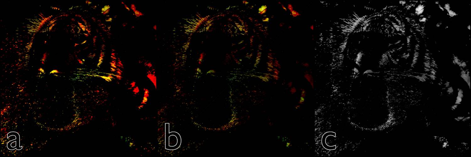
Fig. 6.13) 2 images mixed by the blend type burn . For the original images compare fig. 6.2, For the node setup see fig. 6.1, in b) and c) the inputs for the mix node were switched, in c) the images were desaturated before getting mixed.

This is the inverse of dodge. The formula of this method is similar to the screen mode, but instead of multiplying, the values get divided. Since it is still inverse (1 - x) this effect darkens your image as opposed to the screen method. It will also increase the contrast a lot.
Hue
Fig. 6.14) 2 images mixed by the blend type hue . For the original images compare fig. 6.2, For the node setup see fig. 6.1, in b) and c) the inputs for the mix node were switched, in c) the images were desaturated before getting mixed.
The RGB values will be converted to HSV, then each pixel will get the hue of the lower value, keeping its lightness and saturation. If there is a plain color in socket b, the resulting image will be somewhat tinted in that color. Since altering the hue of a gray value (saturation = 0) does not colorize the pixel, if a pixel in b) has a neutral color, a it will not be altered by this blend mode.
Saturation
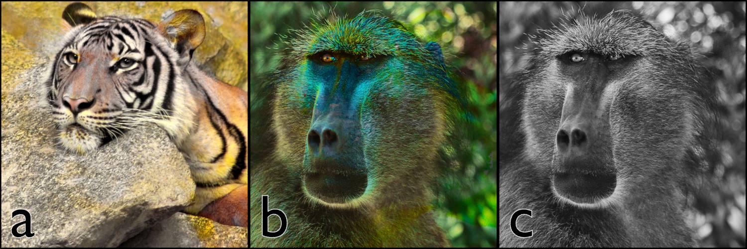
Fig. 6.15) 2 images mixed by the blend type saturation . For the original images compare fig. 6.2, For the node setup see fig. 6.1, in b) and c) the inputs for the mix node were switched, in c) the images were desaturated before getting mixed.
The RGB values are converted to HSV. The resulting color will keep its hue and lightness, but get the saturation of the lower socket. If either one of them is neutral (gray, R = G = B) the resulting pixel will receive a saturation of 0. Hue and lightness of the colors will not be affected.
Value
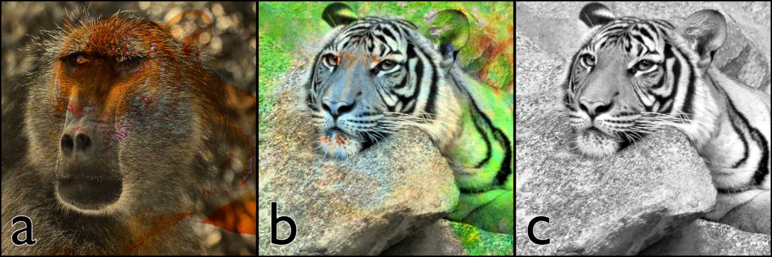
Fig. 6.16) 2 images mixed by the blend type value . For the original images compare fig. 6.2, For the node setup see fig. 6.1, in b) and c) the inputs for the mix node were switched, in c) the images were desaturated before getting mixed.
This mode ignores the color information of the lower image. It will only use the brightness, which is similar to the value in HSV. All pixels will keep their hue and saturation, but receive the brightness of the pixels in the lower socket.
Color
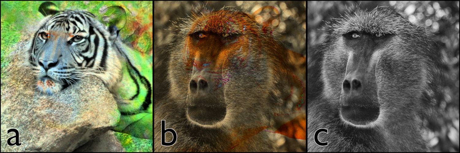
Fig. 6.17) 2 images mixed by the blend type color . For the original images compare fig. 6.2, For the node setup see fig. 6.1, in b) and c) the inputs for the mix node were switched, in c) the images were desaturated before getting mixed.
With this method the ratio of R:G:B will be same as the one in the lower socket. This way the image gets tinted in the color of the lower socket. The maximum saturation a pixel can get is determined by the saturation of the color in the lower socket. The lightness will not be affected. Neutral colors in the lower socket will not affect the image.
Soft Light
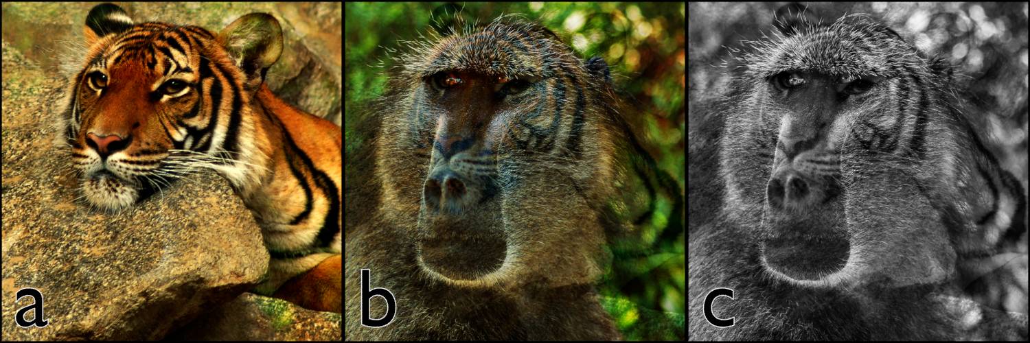
Fig. 6.18) 2 images mixed by the blend type soft light . For the original images compare fig. 6.2, For the node setup see fig. 6.1, in b) and c) the inputs for the mix node were switched, in c) the images were desaturated before getting mixed.

There are several other algorithms to achieve this effect, but they all do something very similar. Essentially it is something very similar to the linear light, but does not alter the image as drastically. There is less increase in contrast.
Linear Light
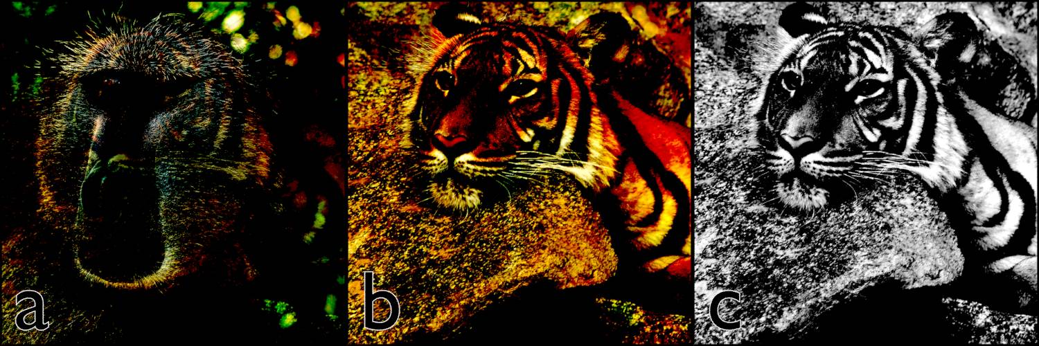
Fig. 6.19) 2 images mixed by the blend type linear light . For the original images compare fig. 6.2, For the node setup see fig. 6.1, in b) and c) the inputs for the mix node were switched, in c) the images were desaturated before getting mixed.

Brighter pixels in a will strongly brighten b) and darker pixels will darken that area considerably, resulting in a strong effect.
Clamp
Will not allow any output value to be greater than 1 or smaller than 0. This can be especially useful if you add two textures and use them for a diffuse material, because providing an input value greater than one will make it act somewhat like a noisy emission material while an input value smaller than 0 will result in a kind of black hole material that is actively removing light from the scene.
Fac
Determines the strength of the effect. Higher values will make the lower color more effective, lower values will leave the upper color unchanged.
Hint: You can use a black and white texture to control the strength of the effect across your model.
Color1 / Color2
The RGB or texture input for the two colors that are supposed to get mixed. The lower socket will be composited on top of the upper one.
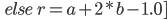
RGB Curves (R)
These curves are very useful as they allow you a fine control on how to transform the color of a pixel depending on its RGB information.
If C is enabled, the X and Y axes both represent the brightness of the pixels. As long as you keep a straight 45 ° line from bottom left to top right, nothing is altered, because for each input value (X) the same output value (Y) is used. You can alter the Y value of each point of the curve. Increasing them will make the corresponding pixels brighter and decreasing them will darken all pixels with the brightness indicated by the position in X.
This way the bottom left corner represents the black pixels, while the upper right represents the bright pixels.
If you click on a dot on the curve, you can move it. If you click anywhere else on the curve, a new dot is created. If you push up the bottom left dot, you will clip the blacks, because the brightness of all pixels with a lightness of 0 (0 position in X) will be increased.
The standard contrast increase method is called a sigma curve . It looks like the letter S (fig. 6.20)
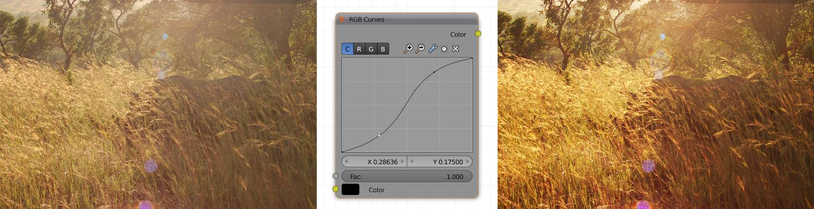
Fig. 6.20) Curves resembling a sigma increase the contrast by brightening brighter pixels and darkening the ones below 0.5.
If you switch to R, G or B, the same principle applies, but instead of X and Y representing brightness, they will separate pixels depending on their R, G or B value.
For finer adjustments of your curve you can use the + to zoom in and zoom out again with the – button. For even more precise control you can click on a dot and adjust its X and Y location with the two sliders you see right below the grid.
If you click on the wrench you can choose from these options:
Reset View
In case you zoomed in or out using the + or – symbol, this will undo those changes and set the zoom to its original value.
Vector Handle
The standard method of interpolating between two points is auto, somewhat similar to Beziér handles, vector handles will result in a linear interpolation.
Auto Handle
The standard method of interpolating between two points is auto, somewhat similar to Beziér, in case you set this to vector earlier, you can use this function to reset it to auto.
Extend Horizontal
The two extend-options only affect the curve before the first and after the last point. For extend horizontal, the curve outside of the first and last point will be horizontal, meaning all points after the last point will get the same Y (transformed) value as the last one and vice versa for the first.
Extend Extrapolated
This is the standard setting, so it will only influence anything if you previously chose Extend Horizontal. This option only does any changes if you move the right- or leftmost point on a curve. If it is set to extrapolate, the curve beyond this point will continue with the incline of the last dot on the curve and vice versa for the beginning.
Reset Curve
Can be used to reset the curves, assigning all points the same y value as their x value is and deleting all manually inserted dots for C, R, G and B.
Clipping Options
Using the little circle you can clip the area in which the dots can be moved, preventing you from moving them too far for your taste by accident.
Delete Points
If a dot is selected, you can delete it with the x symbol.
Fac
How strong the effect is. Typically you will leave this at one, if not the original image gets calculated back into the corrected one. It can be useful however to limit the effect to certain areas using a texture.
Color
Input for an RGB value or a texture.
Invert (I)
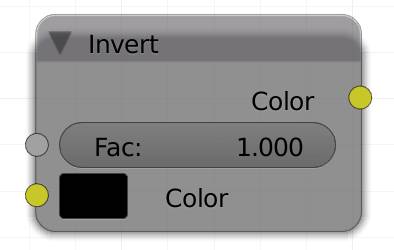
It inverts every pixel, meaning white becomes black, blue becomes yellow, green magenta and red turquoise. This is most commonly used to invert grayscale maps to reverse their influence.
Factor
You can choose a factor, which will pull the two values closer together - figuratively speaking, if they were on a color wheel. A Factor of 0.5 will therefore result in a plain gray color, no matter what the input was.
Light Falloff (L)
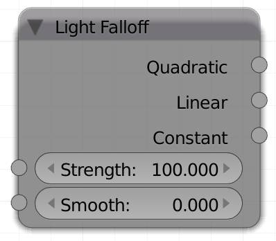
As you can see the output sockets of this node are gray. This indicates that the light falloff node will not output any color information, only variations in lightness.
If an object moves further away from a light source, the amount of light it receives decreases by the square of the distance. Meaning an object that is twice as far away from the light will receive one quarter (2 * 2) of the light. A distance of three times will decrease the light by a factor of 9 (3 * 3).
Sometimes it is nice to be able to change the physically correct ways in order to fit your needs, so you can bend that law using the light falloff node. You can use this node for lamps to alter their native falloff as well as the illuminated object.
Since linear and constant falloff brighten objects more than natural falloff, bouncing light rays can actually increase in lightness therefore the image can be extremely bright if you are using a lot of bounces.
It has two inputs:
Strength
The strength of the light before the falloff effect gets calculated.
Smooth
Surfaces very close to a light source can become very bright and thus a source for noise in a scene. Smooth counters this effect.
And three outputs:
Quadratic
Using this option would be closest to natural lighting behavior.
Linear
Transforms the natural quadratic falloff to a linear one. This means an object twice as far away from the light source will receive half as much light, and not only a quarter as much.
Constant
Ignores the distance from the light source and uses an absolute value that is calculated by dividing the strength by the smooth input. A smooth value of 0 will be ignored and only the strength value will be returned.
Hue Saturation/Value (H)
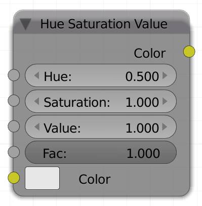
This node can be used to alter the colors of a texture. You can address the HSV properties individually. You can see the effect live if you enable HSV selection on the color picker.
HSV stands for Hue, Saturation and Value.
Hue
A value of 0.5 means no change, so this is where we start off. If you increase the hue, your color picker will be chased along the color wheel clockwise. If you lower the value, the color picker will rotate anti clockwise, however they will not change in brightness. Since 180° to the left is the same as rotating a 180° to the right, a Hue of 0 or 1 will invert the color, but not its brightness or saturation.You can see this effect live if you enable HSV selection on the color picker.
Saturation
This value will determine the distance of your color picker from the center. Since there is no red and blue where green is on that wheel, desaturating green means adding both red and blue, making the result seem brighter. If R = B = G, the resulting color will be gray, so saturation will increase the difference between the R, G and B value of your color.
Value
The value of a color loosely correlates with its brightness. Next to the color wheel in Blender there is a bar from white to black, value does the same thing as sliding the picker up or down the slider. To see the difference between HSV and HSL .
Hint: This effect is much more subtle than the brightness settings from the node, so I usually prefer this method to darken or brighten an image.
Fac
How strong the effect is. Typically you will leave this at one, if not the original image gets calculated back into the corrected one. It is useful however to limit the effect to certain areas using a texture.
Color
Input for an RGB or a texture.
Gamma (G)
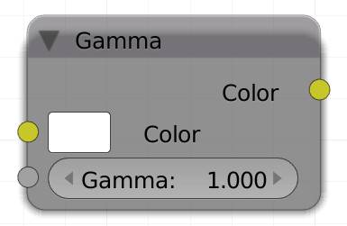
Human eyes have sort of an internal contrast enhancement. Thus reality seen with our eyes has a non-linear lightness perception. Standard cameras do not, so some images can appear kind of grayed out. Gamma correction can be used to make them appear more life-like. The gamma correction therefore is non-linear. The same effect can be achieved by using curves, if you only use a single control point and move it only along a line orthogonal to the default curve.
Color
Input texture to be gamma corrected. I'm writing “texture” instead of color, because it does not make too much sense to input a single color here.
Value
Essentially values smaller than 1 will fade out the colors, making your image to appear brighter and less saturated. High values will darken the image and increase the contrast a lot.
Bright Contrast (B)
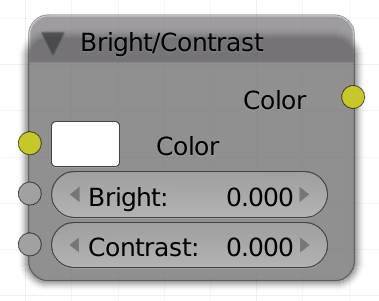
The brightness and contrast node is supposed to let you easily adjust the brightness and contrast of a texture. Unfortunately it produces burnt looking areas even with very small values, so I usually use a hue / saturation node for the brightness and increase the contrast with curves.
Color
Input texture to be adjusted. I'm writing “texture” instead of color, because it does not make too much sense to input a single color here.
Bright
Adjusts the brightness of the texture.
Contrast
Adjusts the contrast of the texture.

