Chapter 17: The Truth about Normals
What are Normals?
When I first started with Blender I read about normals everywhere, but all I knew about them was: If there are weird black spots on your object, go into edit mode and press CTRL + N to recalculate them. But then I stumbled across them in particle systems, texture inputs, and what-not.
So what are normals? Let’s get a little mathematical here. You cannot determine the angle a light ray hits a surface directly. Grab a pen and hold it so one end touches a piece of paper. As soon as you hold it at an angle, there is an infinite number of angles you could measure, all around the pen (fig. 17.1, left), so how do you decide which one to use? The answer lies in the normals of your piece of paper. If you raise the end of your pencil, so it is pointing exactly upwards, you will see that now there is only one angle to be measured: 90° all around, it is a right - or normal - angle. So a normal of a face is any line coming straight from it. It is possible to calculate the angle between two lines , so if a light ray hits a surface, its direction is compared to the normal of the face it hits, and the behavior is calculated from this angle.
A normal also has a second function. By looking at the normal you can determine whether you are looking at the front or the back of a face, because the normal will always point away from the front side.
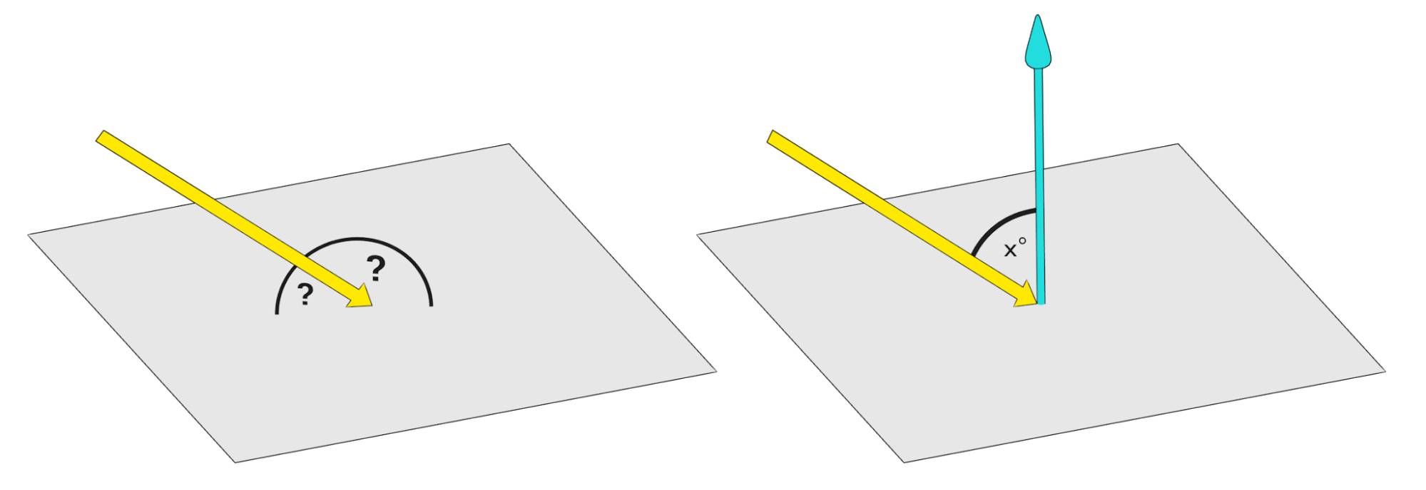
Fig. 17.1) left: It is not possible to tell at what angle an incident ray hits a plane directly. However, you can calculate the angle between two lines. Since a normal is orthogonal to all directions of a face, Blender can draw all vital information about angles from the normals of a face (right).
The cool thing about normals is that you can manipulate them and thus you can change how the renderer perceives the angle of incident rays. That concept is used in smooth shading. Even if a surface has very steep angles, it can be forced to appear smooth by interpolating the normals between vertices . Consider the following example:
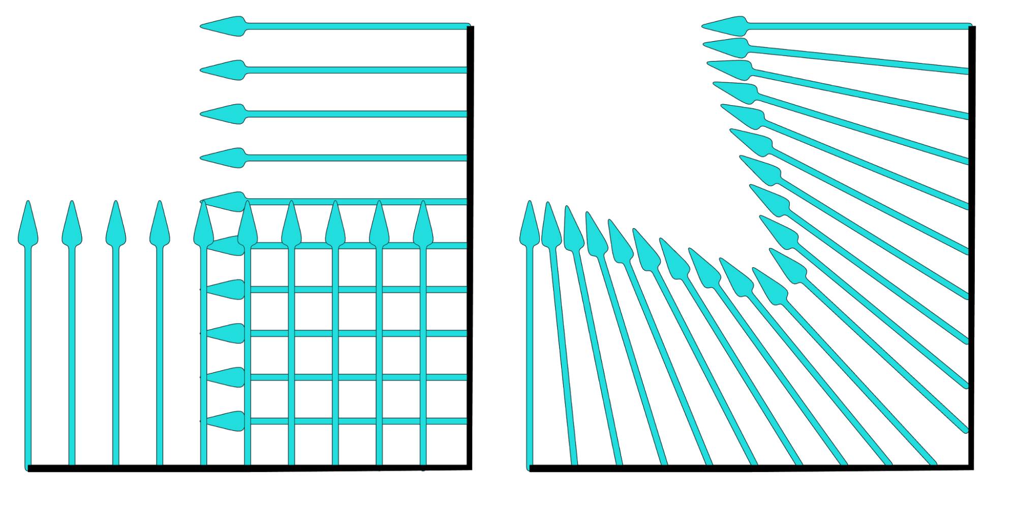
Fig. 17.2) On the left the normals of a corner of an object when shading is set to flat. On the right the same object with smooth shading. The direction of the normals gets interpolated for each shading point.
So by interpolating the normals an angular surface can look rounded. In Cycles, the effect applies not just to the look of a surface but also on the way light is traveling, ie. how it reflects and refracts:
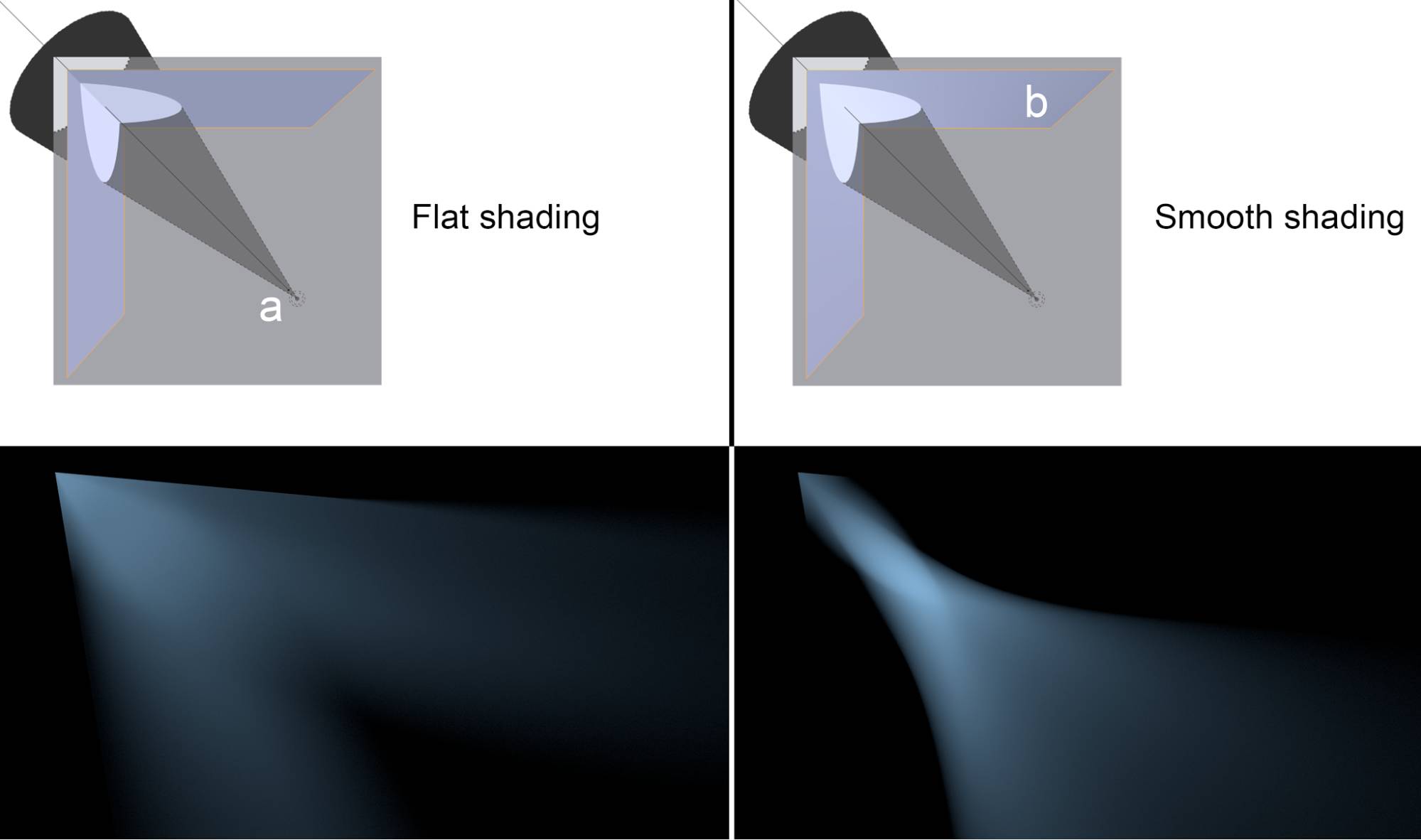
Fig. 17.3) The effect of smooth shading on reflections. On the top the setup - a spot lamp (a), diffuse ground and a model of a corner made from two faces with a set to sharp (b). On the left with flat shading for the corner object, on the right with smooth shading. On the bottom left the corner was set to flat shading. The light was reflected as expected from a mirror. On the bottom right the corner’s shading was set to smooth. You can see that the outline, where the light hit the corner was sharp, but the reflection behaves as if it was produced by a concave mirror.
N ot just faces have normals but also vertices. For vertices the direction of the normal is determined by the adjacent faces. You can visualize them directly in Blender by going into edit mode, then to the properties panel (N-Menu) where you will find symbols to visualize the normals in the Mesh Display section:
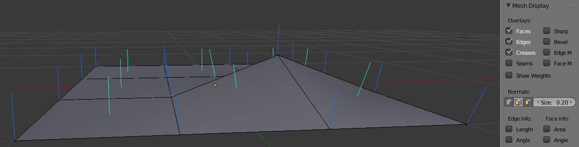
Fig. 17.4) Vertex normals (blue) and face normals (turquoise) visualized in the Blender viewport by clicking on the corresponding symbols under Normals.
Normal Maps
As you can see, the direction of a normal is not carved in stone. Interpolation due to smooth shading is one example where the normals of a surface get changed. But you can also influence the local direction of a normal directly, using a texture or so-called normal map. The three color channels of the texture will influence the three vector components of the normal ( Red: X, Green: Y , Blue: Z ).
Let’s have a look at the math behind normals. As you can see in fig. 17.1, the angle in which a ray hits a surface is determined by the angle of the normal at the exact spot the ray “arrived”, called a shading point. Faces - if shaded smooth - have an infinite amount of normals, but each shading point has only one. So let’s look at that single normal. The angle at which a ray hits a surface is calculated by the angle between the ray and the normal (See fig. 17.1). This and the material settings influence the behavior of the ray after the collision. The easiest example is a perfectly glossy surface, because there is no coincidence factoring in on the behavior of the rays. If it hits a plain surface, its angle of incidence equals the angle of reflection. If you plug the normal output of a into the color of an (node setup in fig. 17.5), you can see the normals expressed as colors ( Red: X, Green: Y , Blue: Z ).
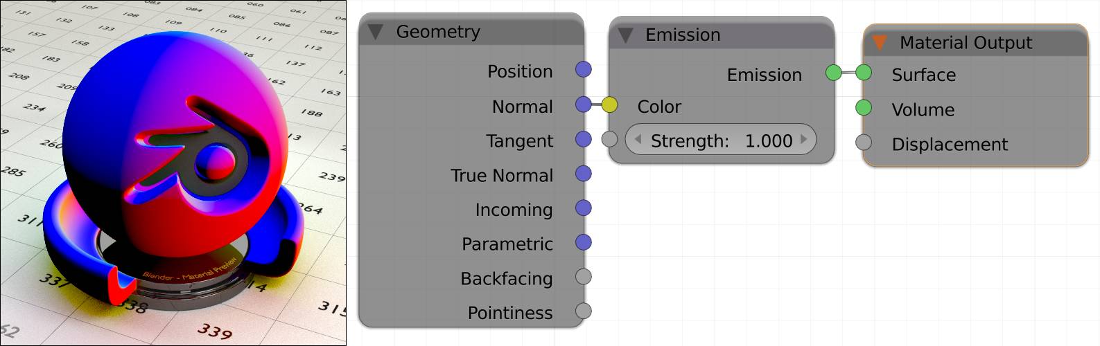
Fig. 17.5) The normals of an object can be visualized by plugging the normal output of the into the color input of an emission shader. Using the you can achieve this quickly by holding Ctrl+Shift and left-clicking the geometry multiple times.
Red denotes the local X-axis, green the Y-axis and blue the Z-axis. On the black parts on the model, all normals point into negative directions.
If you use a node in your material, the angle of individual shading points can be altered, using the color information as vectors (fig. 17.6). So the surface is pretending to point in a different direction than the geometry declares. To determine how much and in which direction the resulting normal is altered, Cycles looks at the color information. Since there is nothing actually sticking out of the surface, it will only work from fairly steep angles (fig. 17.6), but in those cases it actually works pretty well.
The effect of a normal map is more convincing from steep angles as for shallow angles the lack of geometry becomes evident:
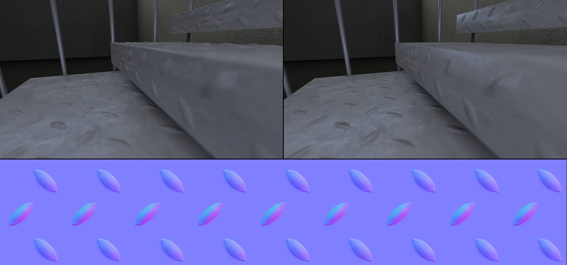
Fig. 17.6) Bottom: An example of a normal map and its application. Top left: A scene with where the bumps were modeled, the stairs consist of 260,000 polygons. Top right: The same scene using a normal map, only 6 faces were necessary. Right: for very flat angles, the missing geometry becomes evident.
The normal map (bottom) was created by placing simple plains under each surface of the stairs and baking the high resolution geometry as a normal map onto them.
The mostly blueish colors you see in fig. 17.6 make up a tangent space normal map, where a value of 0.5 for red (X) and green (Y) is considered straight up and a blue usually has a value of 1.0 as it is only needed for normalization purposes . At a pixel with red, values smaller than 0.5 the normal direction will be shifted to the left, values higher than 0.5 make it point to the right:
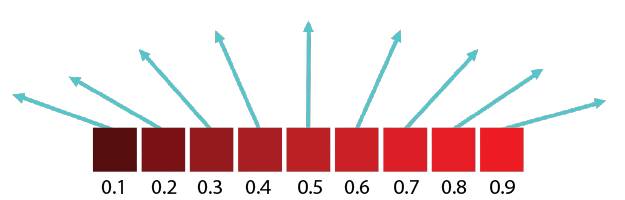
Fig. 17.7) Array of pixels that represent normals, just the red channel. Values smaller than 0.5 make the vector point to the left, values higher than 0.5 make it point to the right and exactly 0.5 is straight up.
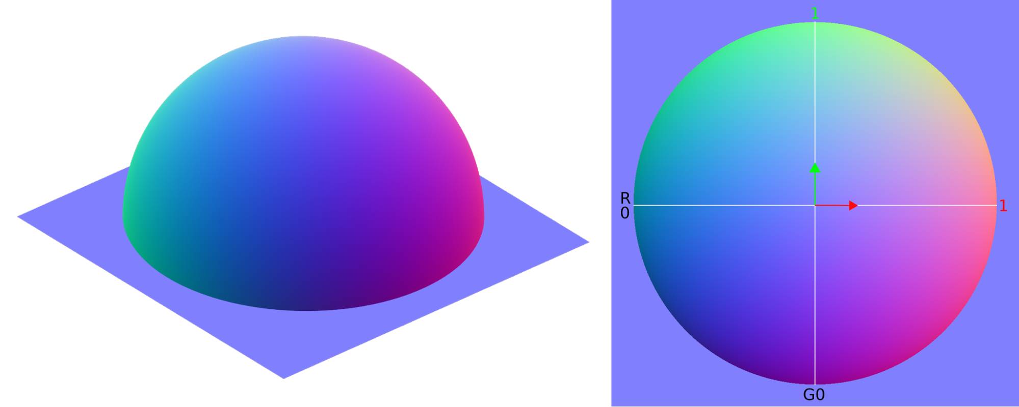
Fig. 17.8) Normal map baked from a hemisphere. On the left the original model with real geometry. The colors represent the direction of the real normals. On the right the baked normal map. The red and green channels form gradients from left to right (red) and bottom to top (green).
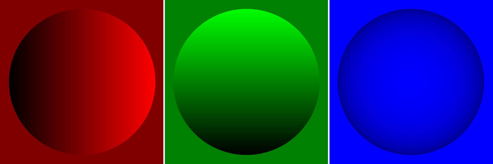
Fig. 17.9) The normal map from fig.17.8 split into red, green and blue channel.
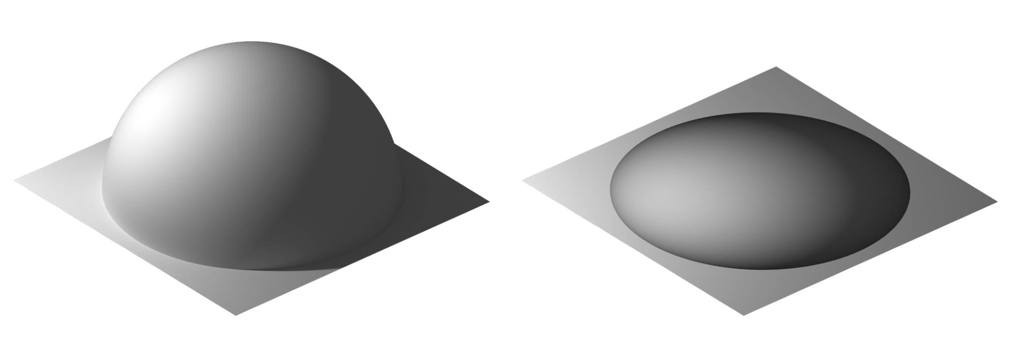
Fig. 17.10) Left: the geometry from fig. 17.8 with a point lamp shining from the left. Right: a plane with a normal map baked from that geometry and the same light setup. Although the light rays were reflected into the correct directions, the silhouette of the sphere is not rendered. Therefore it is not able to cast shadows onto the surface or interact with bouncing light.
The Difference Between Normal and Bump Maps
Bump maps are simple black and white images that Cycles can use to simulate distortion of a surface. White means this part should react as if it was standing out of the surface while black means it gets pushed down. Therefore middle gray is the neutral color of a bump map.
Since it is fairly simple to obtain a grayscale image, but rather cumbersome to bake a normal map, why would we bother to use the latter?
There are 4 key differences between normal and bump maps
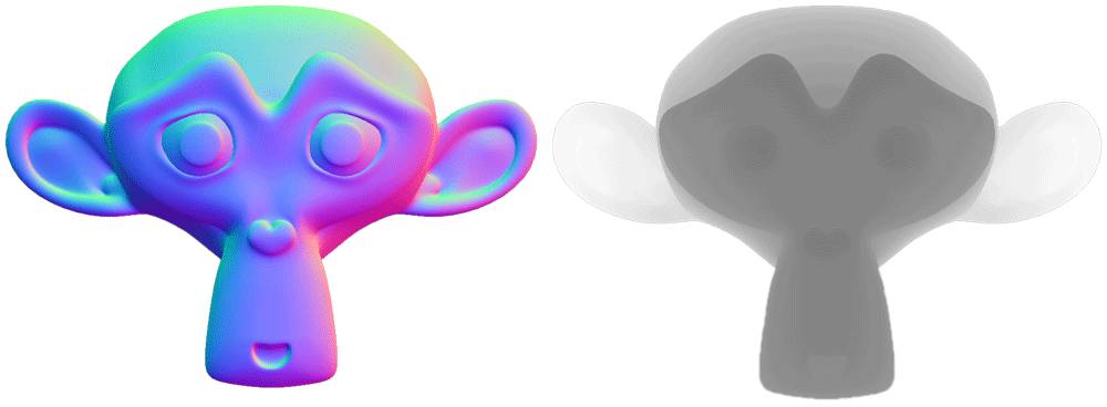
Fig. 17.11) The baked maps for the effect in fig. 17.12 below. Left: Normal map, right: Displacement (bump) map.
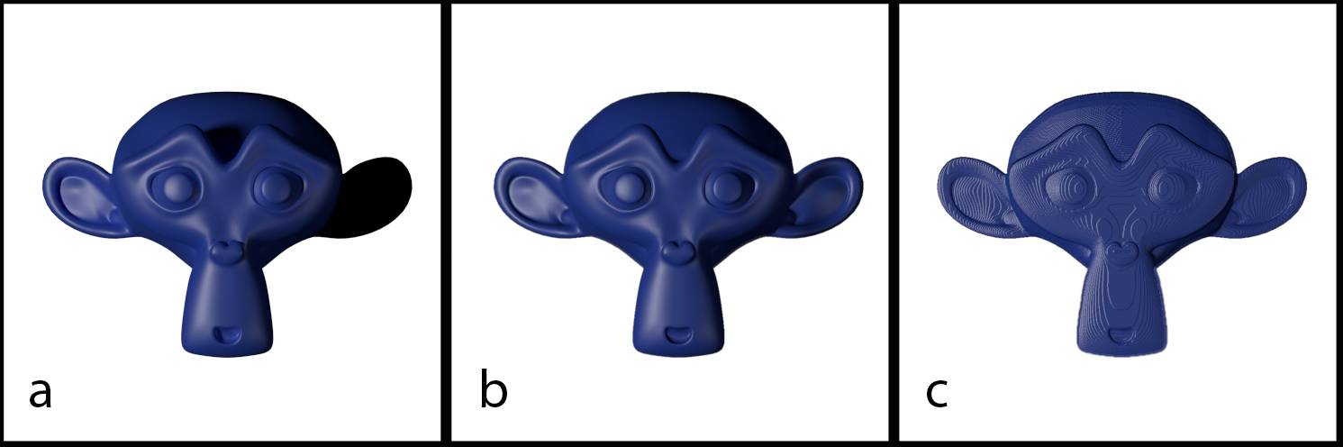
Fig. 17.12) Renderings of Suzanne.
a) actual geometry.
b) Plane with normal map baked from Suzanne.
c) Plane with bump map baked from Suzanne. Note how the light in a reacts very similar as in b, but in b) and c) the object does not cast a shadow on itself. Using a bump map in this situation causes harsh banding (c).
1. While bump maps simulate displacement, normal maps alter the direction in which rays bounce off a surface. As previously mentioned X, Y and Z are more or less equivalent to R, G and B. If a light ray hits a surface the color at this place, calculated by the angle of the shading point towards the camera, is used to determine the behavior of the ray.
2. Normal maps render very fast, because only the color at the according shading point needs to be looked up. With bump maps the difference of neighboring heights needs to be calculated. In Cycles you will not notice the difference, in computation time, but most game engines only use normal maps.
3. The third advantage of normal maps is the precision. Normal maps make use of red and green. In an 8 bit color space that means 256 x 256 = 65536 colors. Bump maps only use a desaturated image, which means there are only 256 different shades available, see fig. 17.11. This inevitably leads to banding as you can see in fig. 17.12 c).
4. So why use bump maps at all?
Even though they provide a lesser range of combinations, they are more suitable for small dents, scratches and especially steep angles. The smallest dent you can simulate on a surface with a proper normal map would consist of 9 pixels, a neutral one surrounded by 8 others that simulate the “walls” of the hole . Also for a normal map it is impossible to simulate 90° angles.
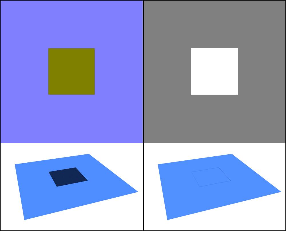
Fig. 17.13 ) On the top you can see a normal (left) and a displace (right) map baked from a cube onto a plane. On the bottom is the same plane, rendered once with the image used in a normal map node (left) and bump node (right).
In Fig. 17.13 you can see that a normal map baked from a cube does produce results that you might not want to get. The greenish color you see results from the method Blender Internal normal baking uses. This also happens in Cycles baking, if you are using the cage option. Rays trying to reach the surface of the plane while baking get blocked. Since the angle of the surface is the same as the plane’s surface, red = green = 0.5 at this point meaning the direction of the normals in this area does not get affected. But the blue value - which is supposed to be 1 at this point - is 0, resulting in a somewhat unpredictable behavior in render. Cycles normal baking without a cage does exactly that, return a blue value of 1, so the color is actually the neutral normals color. This way you would not see any changes in the normal map from geometry facing the same direction as the surface beneath it.
As you can see on the right, in this extreme case a bump map is much more suited than a normal map. Simulating 90° angles with a normal map is not possible, you’ll need to use a bump map instead.

