Chapter 3
Meshes, models and textures
3.1 Structure of 3D mesh objects
3D objects in Blender are often referred to as meshes. Each mesh is fundamentally composed of vertices, lines and faces. A vertex is a singularity construct—it has no volume associated with it—and is defined by its X–Y–Z coordinates in the global 3D view port. These coordinates can be transformed to another coordinate system or reference frame. Vertices can be connected via lines and a closed loop of vertices and lines can form the boundary for a solid, flat surface called a face.
A mesh has geometric properties that include an origin about which the object can rotate and/or revolve. The individual vertices, lines and faces can be edited in Mesh Edit mode, accessed via the Mode Selection drop-down menu or the TAB key (figure ). Each mesh has a selection mode via those vertices, lines and faces.
3.1.1 Example: building a simple model
A base mesh can be created by Add → Mesh from the menu at the top of the screen. The basic meshes are shown in figure . These can be deformed, changed and extended to fit the scientific visualization required.
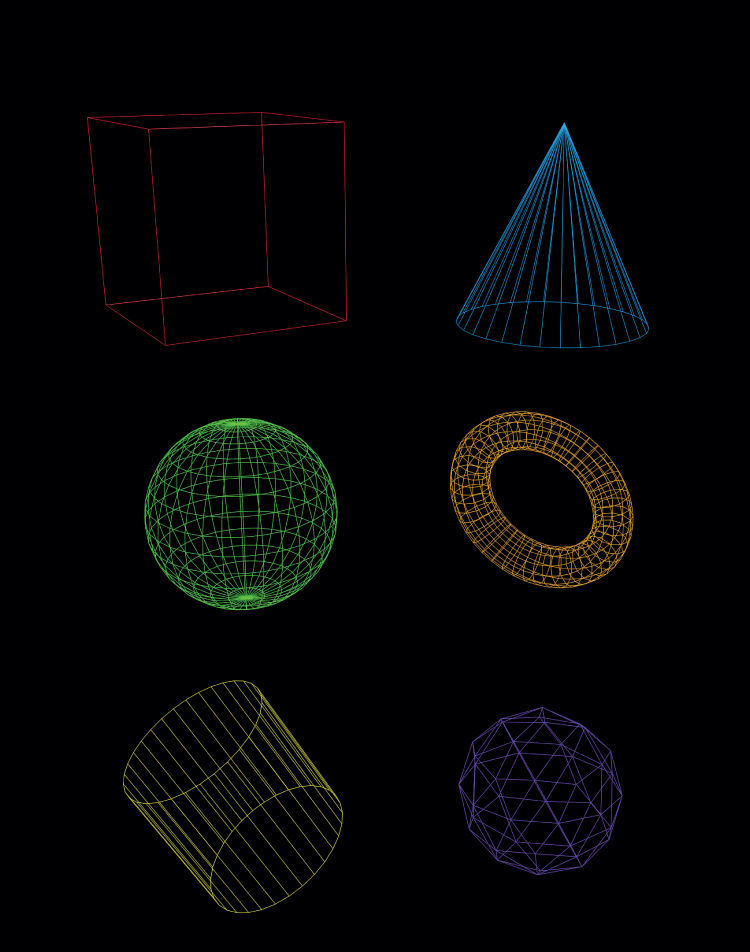
Figure 3.1. Blender mesh examples that form the basis of data containers and grid constructs in scientific visualization. These basic shapes—a cube, cone, UV-sphere, torus, cylinder and icosphere—can be manipulated in the Blender 3D view port.
- Create a new cube mesh by clicking Add → Mesh → Cube. Alternatively, the keyboard shortcut SHIFT–A can be used.
- Rotate the cube with the R key in the plane normal to the line of sight.
- Scale the cube with the S key.
- Translate the cube in the plane normal to the line of sight with the G key.
- The Transform toolbar on the right-hand side of the GUI allows for exact positioning of the mesh object.
We can further manipulate the individual elements of the mesh in a number of ways. This can help the user precisely position the scene elements and data objects of a visualization.
- At the bottom of the 3D view port, click the drop-down menu and choose ‘Edit Mode’. Alternatively, press the TAB key on the keyboard.
- The mesh element faces, lines and vertices will be highlighted in orange. The mode for vertex, line, or face selection is shown in figure . A mesh element can be selected with the secondary mouse button (usually the right mouse button). Multiple elements can be selected by holding down the SHIFT key.
- Groups of elements can be selected by hitting the B key on the keyboard (for box select) and then clicking and dragging a box over the selected points.
- Add vertices connected by lines by CTRL left-clicking where the new vertex needs to be placed.
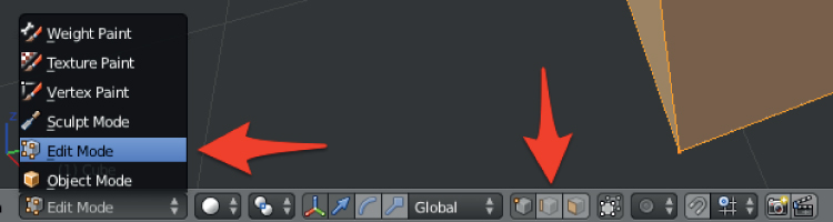
Figure 3.2. Blender Mesh Edit mode is selected and the vertex, line and face mode buttons are shown. This allows the user to manipulate individual parts of a mesh object.
3.2 2D materials and textures
Textures can be applied in a variety of scenarios. 2D textures can be utilized to give a face a more realistic surface appearance, apply mapping data, and change the visibility and color of the data. Bump mapping can also be applied to meshes to simulate 3D surfaces. This has important applications in increasing the speed of rendering times with lower polygon counts []. 2D materials and textures can be applied to single faces or an entire mesh object in a variety of projections in the UV-plane. A orthographic projection map of the Earth is shown in figure and .
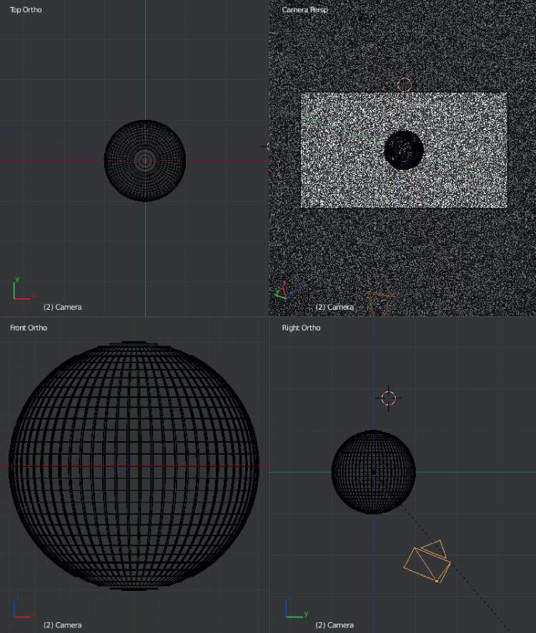
Figure 3.3. This view shows the set-up for projecting a 2D map of the Earth onto a UV-sphere.
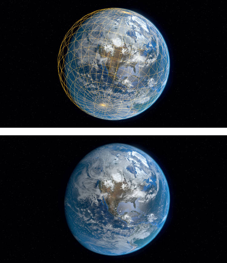
Figure 3.4. Earth map projection with images from . Several layers are presented here in a final composite, including a day and night side maps of the Earth and an atmospheric layer.
3.2.1 Example: adding a texture to a sphere
We can use the following procedure to project the map onto a sphere. This requires marking a seam on the sphere where the object will be separated. A projection of the mesh can then be matched to an image or a map.
- Create a UV-sphere mesh by clicking Add → Mesh → UV Sphere. Alternatively, the keyboard shortcut SHIFT-A can be used.
- Increase the number of polygonal faces for the sphere.
- Select Mesh Edit mode by pressing the TAB key
- Right-click on vertices along a meridian going from the north to south pole of the sphere.
- Press CTRL–E on the keyboard and select ‘Mark Seam’. The seam will be marked in red and show where the 3D object will be separated (figure ).
- Choose the UV-editing menu and open a new image file (ALT–O).
- Select all vertices (A key), press the U key for UV Mapping and select ‘Sphere Projection’ (figure ).
- The results can be see by selecting ‘Texture Mode’ under the ‘Viewport Shading’ drop-down menu.
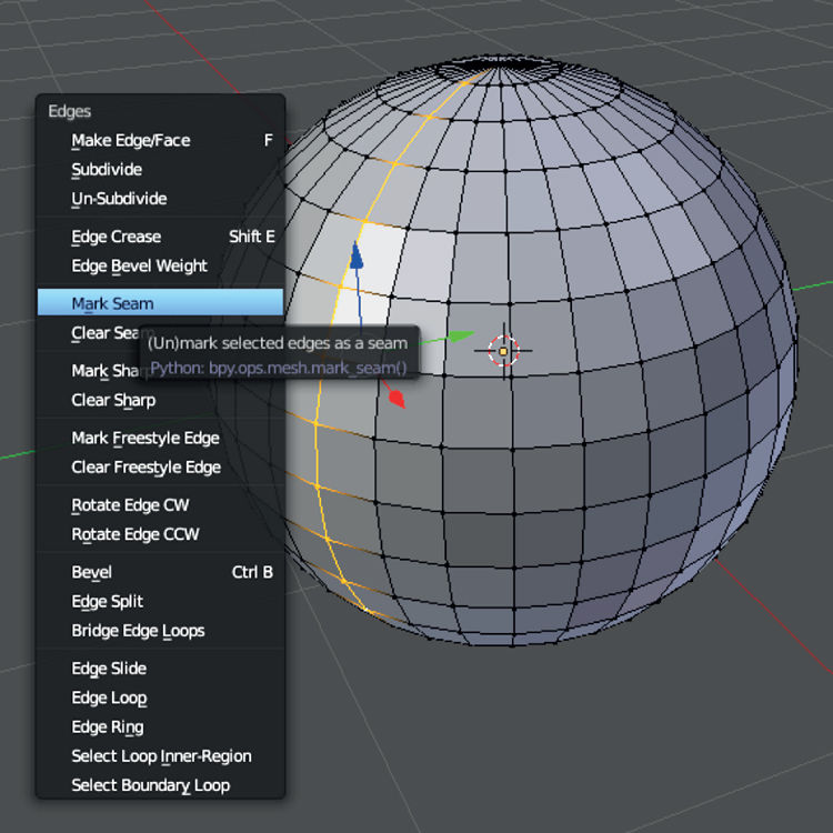
Figure 3.5. In Mesh Edit mode (TAB key), a seam can be added with CTRL–E. In this particular example we are marking the seam along a meridian.
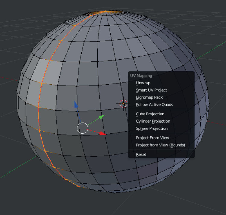
Figure 3.6. With the seam on the meridian properly marked a map projection can now be applied using UV Mapping.
3.3 3D materials and textures
For 3D materials and textures, Blender can apply halos to data points or render data cubes as transparent volumes. Halo textures can be applied to vertices and are useful for creating 3D scatter plots.
3.3.1 Example: creating points for a 3D scatter plot
We will use the vertices of a 3D mesh as our sample X, Y, Z data and texture those points with a halo.
- Create a UV-icosphere mesh by clicking Add → Mesh → Icosphere. Alternatively the keyboard shortcut SHIFT–A can be used.
- Go to the Materials tab on the Properties panel and click ‘New’ to add a new material.
- Select the ‘Halo’ option (figure ).
- Change the halo parameters: size to 0.050 and hardness to 20.
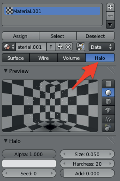
Figure 3.7. The halo material can be applied to illuminate individual vertices in a scatter plot or catalog. These small Gaussian spheres have size, illumination and color properties that can be adjusted.
3.3.2 Example: creating a wireframe mesh
With the same icosphere mesh object (or any mesh), a 3D wireframe object can be created. These are useful for creating background grids in 3D scatter plots. Simply change the material to ‘Wire’ and the shading emission to 1.0 (figure ).
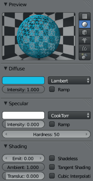
Figure 3.8. A wire material can be applied to a mesh. This is useful in creating grids and bounding boxes for visualizations.
- Create a plane mesh by clicking Add → Mesh → Plane. Alternatively, the keyboard shortcut SHIFT–A can be used.
- Enter Mesh Edit mode by pressing the TAB key on the keyboard.
- On the Mesh Tools panel (left-hand side of the GUI), click ‘Subdivide’ five times to increase the number of grid points in the plane.
- Press the TAB key again to re-enter Object mode. Scale the object to a larger size with the S key.
- Go to the Materials tab on the Properties panel and click ‘New’ to add a new material.
- Select the ‘Wire’ option (figure ). Change the color if desired.
- Change the wire material parameters: Diffuse Intensity: 1.0, Specular Intensity: 0.0 and Shading Emission: 1.0.
Bibliography
[1] Blinn J F 1978 Simulation of wrinkled surfaces SIGGRAPH Comput. Graph.
For excellent tutorials on both novice and advanced Blender usage visit .

