Chapter 1: Introduction
General Notes
With the Cycles render engine you will have 77 material nodes at your disposal. Who could possibly remember them all? Well - you can, with the help of this book.
The letter you see in braces behind the name of a node in this book is the shortcut to select this node from the list your mouse hovers over. Sometimes these get changed by the developers. The shortcuts in this book are conforming to Blender 2.77.
Most Nodes have input and output sockets. In the beginning of the description of a node you will find an explanation what the node does and in the end you will find a list with a shorter description for each socket as a summary.
Those in- and outputs are color-coded, to indicate whether it makes sense to connect two sockets or not. You can connect sockets with different colors, but the effect usually is not what you would expect.
Here is the code:
Blue
This indicates that the socket is a vector, so in other words a list consisting of three numbers which in a coordinate system represent X, Z and Y in that order. Coordinates can also be regarded as color information where RGB represents X, Y and Z.
Gray
Gray inputs take grayscale information and numbers, which are the same internally.
Yellow
These inputs use any kind of color information, RGB, textures or vertex colors.
Green
Those are shader sockets. All shader nodes have a green output, but only mix, add and output nodes have green inputs as well. If you plug anything other than a shader output into a shader input, it will be treated as a shadeless black material.
Nodes can be thought of as little machines . You feed them a raw material and they output some manufactured or altered product. The code above illustrates what they want to be fed, and of what type the product will be. They are fed via pipelines called threads or noodles.
So, How Do I Use Nodes in Blender?
To enable the usage of nodes you need to open a node editor window. Or you can use the compositing layout, it features a node editor and other useful windows all at once. You can switch to the compositing layout by either pressing CTRL + LEFT ARROW or selecting it from the list (fig. 1.1, a). By default this is set to the compositing nodes. These are nodes that alter the image after it is done rendering. At the bottom of the window you can choose between shader, compositing and texture nodes. Click the red sphere to get to the material nodes (fig. 1.1, b). While there are a few nodes the shader nodes have in common with the compositor or texture nodes, only the former will be covered in this book.
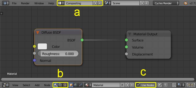
Fig. 1.1) Blender node editor, a) use nodes is enabled, b) node type switched to material (red sphere)
To actually start using the material node editor, there needs to be an active object with a material assigned to it. If you still do not see any nodes, you might have to check “use nodes” (fig. 1.1, c). If this option is not available but there is a button with a + on it that reads “New”, click the button first. A new material should be created and the option “use nodes” should become available. The default material in Cycles has a diffuse shader and a material output node connected to it, resulting in a - you guessed it - diffuse material.
Note: If nodes appear, but they don’t look like in the image above, check whether you have Cycles selected as render engine.
To add a new node, it is probably easiest to hit SHIFT + A. This will make a list pop up just where your mouse cursor is. The list will stay there until you either select a node, or move the mouse away from it. Once you choose a node, it will be added to your material in grab mode. This means, it will move with the mouse until you confirm its position with a left-click. Once you inserted a node, you need to connect it to the rest via a thread, which in Blender is also called a noodle. There are several ways to do that. You can click on an output (dots on the right hand side) and drag a thread to an input of another node (dots on the left hand side). Or you select one node, then hold SHIFT and click on another node and press F. The latter will connect the first two sockets with the same type. So if the left node has an output named “color” and the right one has an input with the same name, they will be connected. Hitting F multiple times will work until all possible pairs are formed.
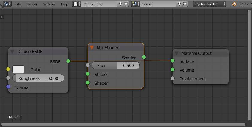
Fig. 1.2) Dragging a node over an existing connection (noodle) will make it turn orange
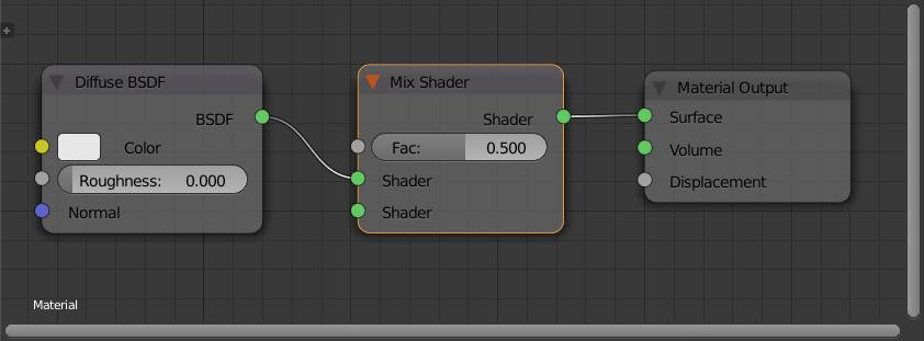
Fig. 1.3) Releasing the node will make Blender guess what connection makes the most sense.
If two nodes are already connected, you can drag a third one over the connections between them. If the compositor finds a combination it considers useful, the thread between them turns orange (fig. 1.2) and if you confirm the node’s position at the point, the new one will be inserted between the two existing ones, already connected to both of them (fig. 1.3). This can be a huge time saver when connecting nodes.
Basics of the Node Editor
The read direction of the nodes is from left to right. This means the left dots of a node are the inputs and the right ones are outputs.
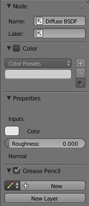
When you press N, the properties menu of the node editor will open. Here you can modify some settings for the active node and the node editor in general.
Node
Under the node properties you can choose a name and a label for the active node. The name is more important for , it is a unique identifier, so each node can be called via Python.
The label is what actually will be displayed as the name of the node in the compositor. If left empty, the type of the node will be used as the label.
Color
To keep things nice and organized, you can colorize individual nodes. To do so, select it and tick the checkbox next to color. After that you can choose the color the node is going to be displayed in. Using the plus you can store a preset, so you can easily assign the same color to different nodes.
Hint: Hovering over a color field and pressing CTRL + C stores the color in the clipboard, and hovering over a different color field and pressing CTRL + V pastes the color there.
Properties
A list of all inputs of the active node is displayed here. If an input is not connected, its values can be altered there, as well as directly on the node.
If you enable the addon, you will get a lot more options in the tool shelf (T).
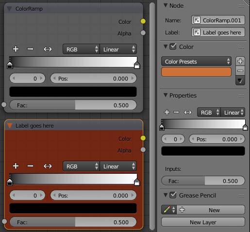
Fig. 1.4) Two ColorRamp nodes. The top one with default settings, the bottom one got a custom label and a custom color. The actual color of the node is darker and more saturated than the color set in the color field.
What You Need to Know About the GUI
In some parts of this book, we will be referring to certain parts of the graphical user interface. Experienced users may know where to find - say, the camera properties - immediately, but just in case, here is a summary of the most important parts. Of course Blender is very complex, so we will focus only on the parts that are relevant for Cycles users.
The Properties Editor
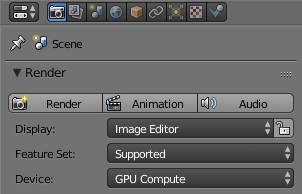
In the default layout, the properties editor is on the right hand side of the screen. The content is context sensitive. This means, depending on what object is active, the menu changes. You can make an object the active one, by right-clicking on it in the viewport. While this might confuse newbies, it is an unconventional, but very effective way to keep the UI lean. This book will only cover the tabs of the properties that are important for Cycles: render, render layers, , object, material, and . For details on the render tab, refer to .
Render Layers
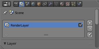
The render layers are very powerful when it comes to post processing. In Blender you can alter the image after it is rendered, you can do color corrections and have a bunch of filters at your disposal. For the purposes of this book, the most important thing is that you can enable the in this tab. The rest is a bit off-topic to be covered in a Cycles encyclopedia.
World
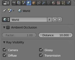
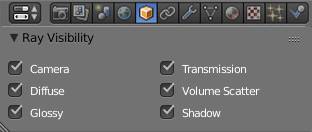
In the world tab you can set the environment for your scene. You can set the distance here. The is special, because it is not bound to one or more objects, but rather to your whole scene. You can specify some of the properties here, like the ray visibility. If you uncheck any of these, the world will not be visible for the according rays. For example, if you uncheck camera, the world will be rendered black when you look directly at it with the camera. But it will still be visible in reflections, unless you uncheck glossy, too. This way you have full control over the behavior of your world material.
Object
Just like the world, objects have a setting, too. You can also turn on viewport transparency for ind ividual objects here. The amount of viewport transparency is not a property of the object but of the material and thus set in the material tab. You can also control whether an object has and the type of motion blur.
Data
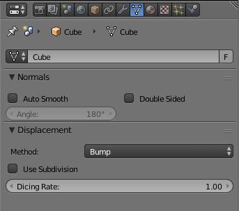
Under the data tab you can find settings about UV maps, vertex color maps and most importantly for this book, the displacement settings. It is symbolized by a triangle mesh.
Note: Displacement settings will only show up when the experimental feature set of Cycles is turned on (see , sub-section Feature Set ).
Material

In the material tab you can manage the settings for the materials assigned to the active object.
To assign a new material, you need to press the plus sign. You can use as many materials as you want for an object, but to actually make any other material than the first visible on your object, you need to assign it to a certain region in edit mode. You can replace the material of an object by clicking the drop down menu marked with a red sphere next to the material name. A list with all materials in the blendfile will open where you can start typing the material name, or use the scroll wheel to go through all of them, until you click on the one you were looking for. If you are new to Blender it can be a bit confusing to edit materials that are shared by more than one object. If so, a number will appear next to the F, which is on the right side of the material name. The number indicates how many objects share the same material. If you change anything on it, the changes will be passed on to all other objects with this material assigned. If you want to change only the material on this particular object, you need to make it a single user. Do so by clicking on the number. Blender will create a copy of it, with “.001” behind the name. Now changes will only affect the current object.
Lamp
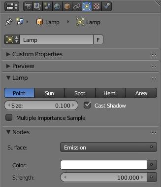
If your active object is a lamp, the material options turn into lamp options.
Since lamp objects usually do not require an extensive node setup, it might be easiest to address their attributes from this panel.
For more details about lamps see .
For more information about the lamp material see the .
Camera
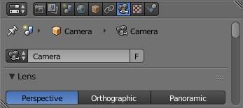
If you right-click on a camera in your scene, the properties panel will include a film camera symbol. this is where you can set all the relevant attributes of your camera. Since Blender is creating an actual environment, it will be perceived through a camera, so there are quite a few parameters to fiddle with here. For a detailed explanation check the .
About the Test Scene
The scene is called b.m.p.s. - Blender Material Preview Scene. It was created by Robìn Marin and released under the creative commons license. It was altered to fit some of the requirements for the test renders in this book.
- The entire scene was scaled down until the test object had a diameter of approximately 1 Blender Unit (BU). Subsequently the grid now had a size of 0.4 BU.
- We added a grayscale HRDi for environment lighting and altered the lamp settings. The strength of the background was left at 1 and the brightest pixels of the image were about 2.7 for R, G and B.
- There are 3 mesh lights in the scene, one shining from the left with a strength of 5, one with a strength of 8 slightly offset to the right of the camera and one that is stretched to be less square with an intensity of 14, but much further away.
- To counter fireflies, caustics were disabled. The Bounces were left at the standard settings for Blender 2.71:
- Max: 12, Min: 3
- Diffuse: 4
- Glossy: 4
- Transmission: 12
- Transparency Max and Min: 8
- Volume: Bounces: 0, Step: 0.1, Max: 1024
- With the exception of hair and subsurface scattering the color of each shader was set to a powder blue (89B2FF).
In case a render was done with a modified version, it is mentioned in the image description.
The scene can be
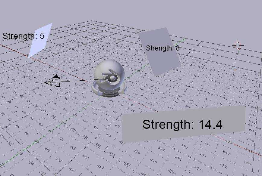
Fig. 1.4) b.m.p.s. overview. The three planes are mesh lights with the light intensities 5, 8 and 14.4, their colors were pure white. The test object had a diameter of approximately 1 BU and the camera had a focal length of 85 mm. The grid size is 0.425 BU.
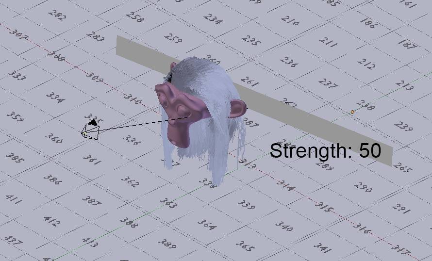
Fig. 1.5) b.m.p.s. modification for hair rendering. Since the translucency for the strands with a transmission shader is fairly weak, we placed a strong backlight (strength: 50) right behind the head, and deleted the rest of the lights. The rest of the settings were left as described above.
Helpful Keyboard Shortcuts
When you are using the Blender node editor, it can speed up your workflow if you are familiar with a couple of shortcuts. Keep in mind that the shortcuts are context sensitive, so if your mouse is not over the node editor, they will do different things.
SHIFT + F3 : Turns the window your mouse is over into a node editor
SHIFT + A : Opens the menu to insert a node.
SHIFT + D : Copies the selected nodes, keeping the connections between them, but not the input connections of the leftmost nodes in the selection.
CTRL + SHIFT + D : Copies the selected nodes, keeping all the connections between the selected nodes.
ALT + D : Disconnects the selected nodes without destroying other connections.
CTRL + X : Deletes the active node, but keeping the connection between the left and the right one of the deleted node.
CTRL + J : Add a frame around the selected nodes.
M : Mutes a node, meaning it treats the node tree as if the node wasn’t there.
CTRL + H : Turns the unconnected sockets on and off.
SHIFT + L : Selects the next node(s) linked to the current one, downstream (meaning if it has a noodle from left to right)
SHIFT + LMB + drag : Adds a to the noodles you dragged across.
CTRL + LMB + drag : Cuts the noodles you dragged across.
Home/Pos1 : Zooms out so your entire node tree fits the screen.
SHIFT + = : Aligns all selected nodes vertically, so the all have the same x-position.
SHIFT + G : Lets you select Nodes that are similar to the one that is active, you can choose:
Type: All nodes of the same type, e.g. Color Mix (no matter if they are set to mix, multiply etc.)
Color: All nodes sharing the same custom color.
Prefix: The first letters that are separated from the name of the node (not the label) by either a
“.” or a “_”.
CTRL + F : Find node, opens a list containing all nodes of the current tree that you can filter by
starting to type either their name or their label.
For more options to speed up your workflow, see the addon.
The Difference Between a Shader and a Material
While reading this book you might find yourself asking: Why does it sometimes say “shader” and sometimes object attributes are referred to as “material”. This is due to an odd naming convention in Blender. Everything that defines the appearance of a surface or volume is a shader in CG terms. Cycles differentiates between “shader” and “material”, though.
“Shaders” in Cycles refer to the shader nodes of the add menu in the node editor. The whole of the nodes, which can contain several shader nodes, make up the actual material.
Cycles vs. Blender Internal (BI)
There is a huge difference between a path tracer like Cycles and a rasterize or REYES renderer like we find in the good old Blender internal renderer or computer games. Cycles simulates a photo camera, tracing light rays as they are traveling through the scene similar to how they would do in the real world ( ). Blender Internal is somewhat like an automated painting application, but in 3D. It gathers scene information and based on that it paints gradients onto the objects in the scene. Reflections and refractions in BI are added on top of that by means of ray tracing, making it a hybrid renderer. That is also the reason why reflections and refractions take a lot longer to calculate in BI. In Cycles the light rays get traced anyways, so reflections are just a different behavior of light bouncing off surfaces.
This also means that materials and shaders differ greatly between Cycles and BI. For Cycles, shaders are definitions how the traversal of light is changing when it hits an object (scattering, refraction, absorption etc.) while for Blender Internal the geometry is shaded roughly according to the environment. In BI, a diffuse surface is just a gradient painted onto the screen and a glossy highlight (specular) is basically a blurred dot painted on top of it. In Cycles, diffuse and glossy are just two different kinds of light scattering definitions and physically accurate.
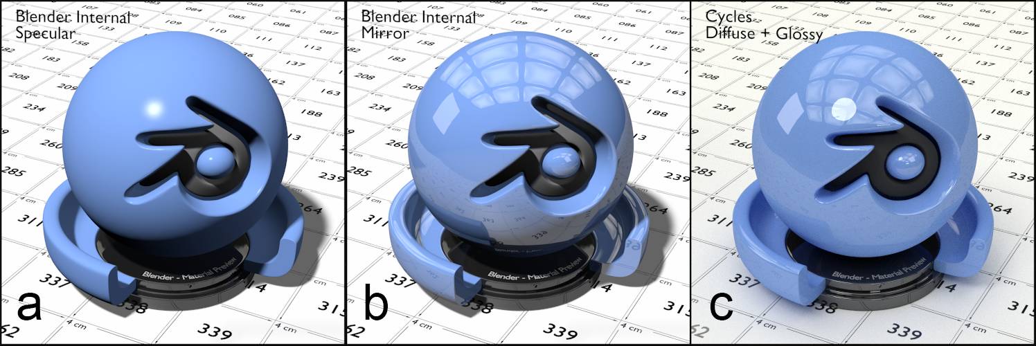
Fig. 1.6) Rendering of the same object with Blender Internal and Cycles renderer. For lighting the same sun object as well as the same image for the environment map was used for all 3 renderings.
a and b) The entire scene was converted to BI materials. The mesh lights were set to a standard material with the according emission values.
a) BI material with a specular intensity 0.6 CookTorr.
b) specular intensity of 0 and mirror enabled with reflectivity of 0.1.
c) Cycles diffuse shader with a mix of 0.1 with a glossy white shader with a roughness of 0. In this case all the mesh lights were set to be visible by reflection only and the scene was lit by the sun and the environment map only.
Note that the object in fig. 1.6 gets illuminated from below when rendered with Cycles (c) while it does not in Blender Internal. This is because BI does not support global illumination. For the specular in Blender Internal only the location of the specular needs to be calculated once, the size and hardness are taken from the material settings. The specular reflection is actually a cheap trick by Blender Internal to get some very basic reflections without increasing render time too much. For actual reflections one reflection ray per shading point is necessary to accurately add them to the material, which obviously takes a lot longer. This is why specular and mirror are also separated in Blender Internal, while in Cycles lamps show up in glossy materials thus there is no need for specular, (b) took 25% longer to render, while in Cycles sharp reflections actually become noise free much faster than diffuse materials do. Rough (blurred) reflections in BI take even longer, while - again - in Cycles there is not much difference between smooth and rough reflections other than how the light rays react when hitting the according surfaces.
Ho w a Path Tracer Works
To understand the drawings in this and the following chapters, it is essential to understand how path tracers in general and Cycles in particular, work. For each pixel a ray is cast into the scene. It starts as a camera ray until it collides with an object. If a surface has an emission or holdout shader, the ray will be deleted and the pixel will receive the color of the emission shader or become transparent. In all other cases the further behavior of the ray is going to be influenced by the type of shader assigned to the surface it hit. The easiest example would be a sharp glossy material. In this case the ray will be reflected by the simple rule of angle of incidence equals angle of reflection. The ray will then continue as a glossy ray. Let’s say after that it hits a diffuse surface. From there it will bounce into a random direction. Assuming that the maximum number of bounces in your scene is not reached before it, the ray will eventually hit a light source. It will be discontinued and the color of the sample the ray belongs to will be calculated depending on all materials the ray hit while bouncing. This process is repeated as many times as you set the number of samples in the render tab. In the end the mean value of all samples is used for the color of the pixel.
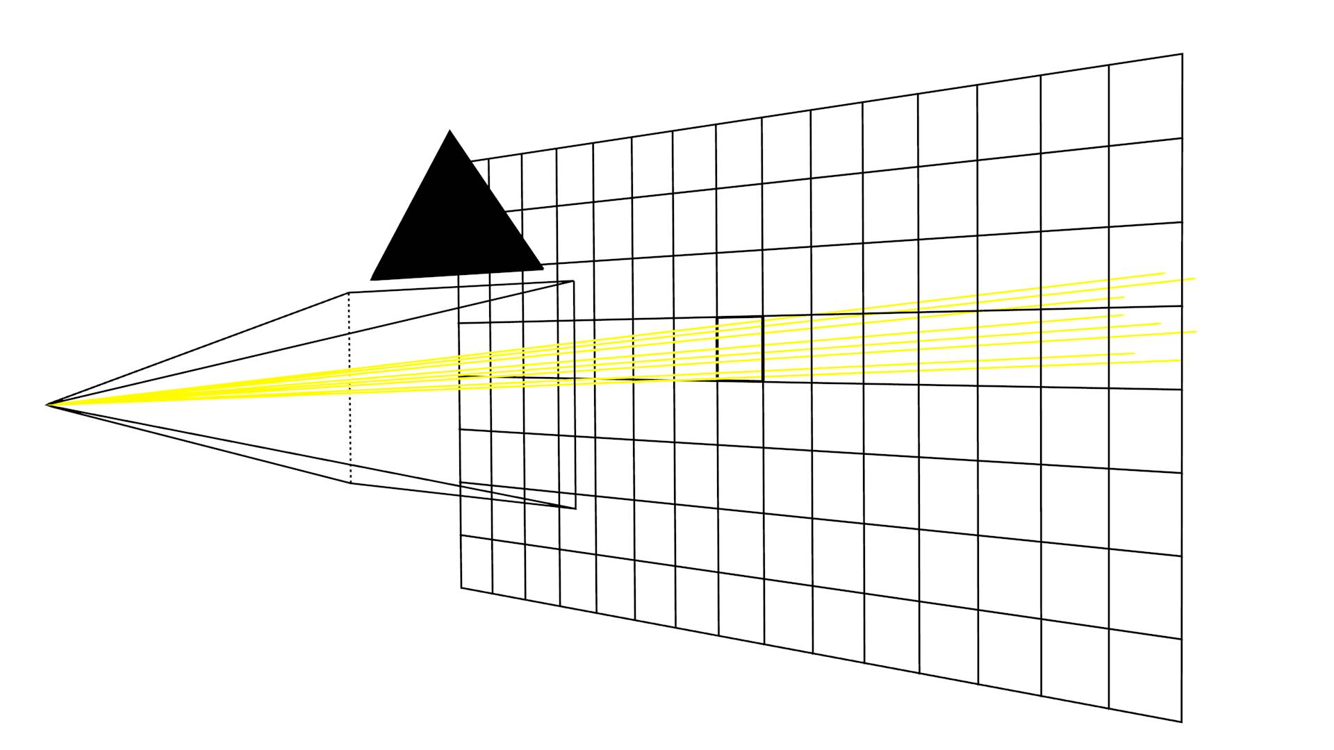
Fig. 1.7) Grid representing single pixels. For each pixel, the rays are fired from the camera into the scene. The number of rays per pixel is the number of samples in the sampling section of the render tab.
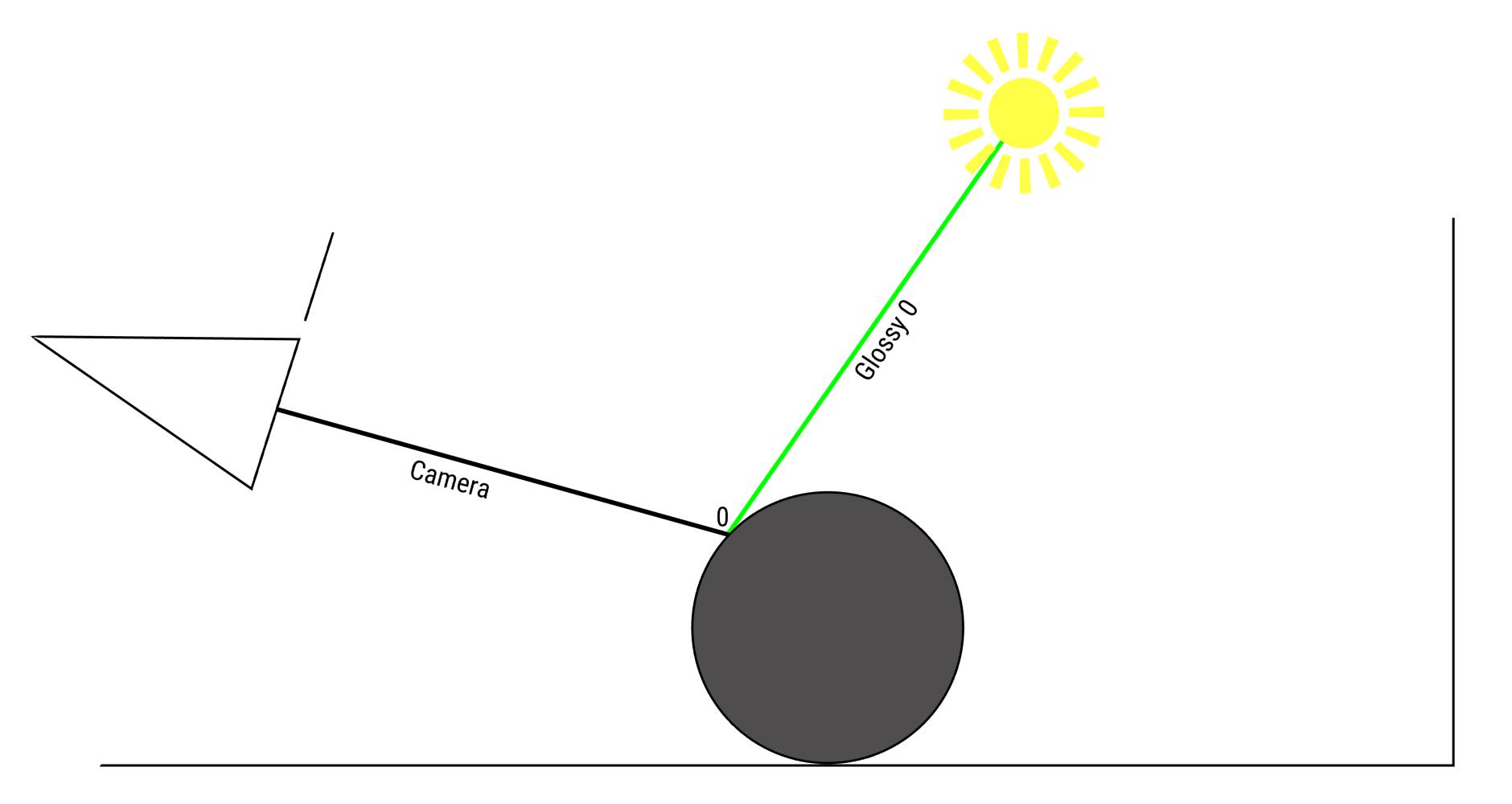
Fig. 1.8) A ray originating from the camera, hitting a glossy object and bouncing off it. Next it hits a light source and thus gets terminated. The ray will return the light information from the light source, minus possible absorption happening on the sphere.
Figure 1.8 shows a very simple case of a ray from the camera hitting a glossy object, bouncing off it and hitting a light source next. This is a very simple example and it will get more and more complex the more features and shader types we add until we get an example close to an actual scene in Cycles. The path after the ray has bounced off the sphere has a green color and reads Glossy 0 . That indicates that the ray has changed from a camera ray into a glossy ray. The 0 denotes that it is the first glossy bounce the ray has encountered (Cycles starts counting at 0). After a ray has bounced off a surface, it changes its type depending on the type of shader that it found on the surface. In this example it was a glossy one. But a different ray from the camera could have bounced into a different direction, hitting the floor which in this example has a diffuse shader. In that case the ray that has bounced off the floor would become a diffuse ray, see fig. 1.9.
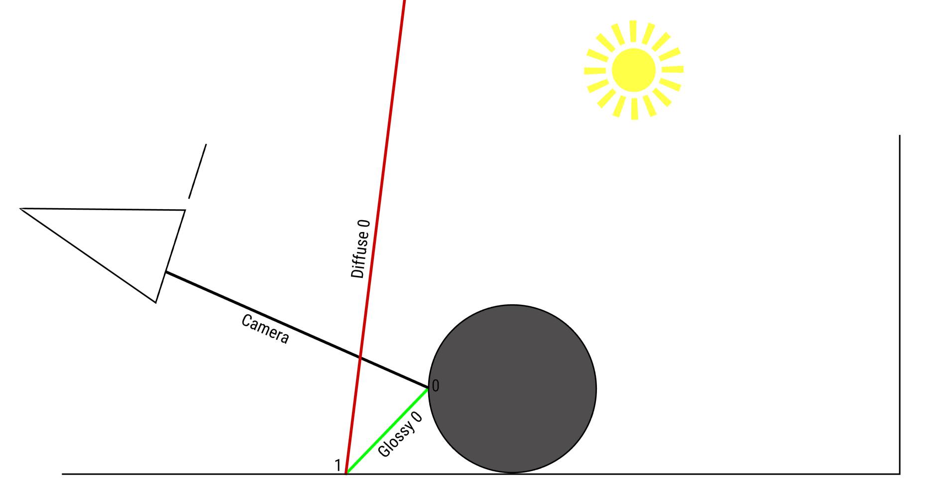
Fig. 1.9) A ray originates from the camera, hits a glossy surface and afterwards a diffuse one. Thus the ray changes from camera to glossy to diffuse.
In the previous examples the object had only one shader and we assume it’s a glossy one. But what if a material uses multiple shader nodes, like almost all materials do? A simple case is a mix of diffuse and glossy or the glass node, which internally is a mix of refraction and glossy. In that case Cycles will randomly pick a shader from the material. If a mix node is used, shader nodes with a higher mix factor are more likely to be chosen and so are shaders that have a brighter color. So let’s change the glossy sphere from the example to a glass one and see what happens (fig. 1.10).
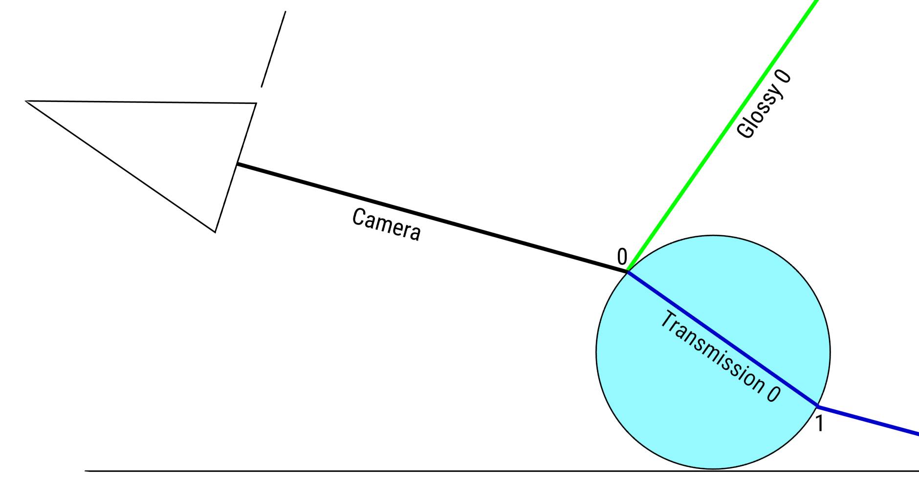
Fig. 1.10) A ray originates from the camera and hits an object with multiple shaders. In this case it is a glass shader, which internally is a combination of refraction and glossy shaders. So the ray now has two paths it can travel.
So actually quite a lot can go on in even a very simple scene. Rays are bouncing around, hitting objects and decide which paths to take. Let’s take a look at an example with two possible routes and see how Cycles is counting bounces (fig. 1.11).
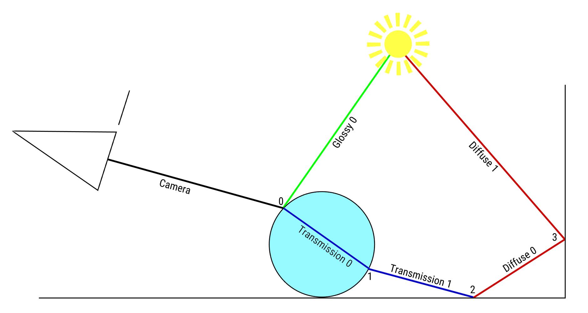
Fig. 1.11) Example of a path a ray can take. It is originating from the camera (black) hitting a glass object. It will then choose to follow either the glossy ( green ) or the transmission ( blue ) path, because glass is a mix of glossy and refraction shaders. At bounce #1 the ray could have reflected off the inside of the glass as well, this was omitted for the sake of simplicity. After hitting a diffuse surface the ray is regarded as a diffuse ray ( red ).
In figure 1.11 you can follow the journey a light path can take. It always originates from the camera, because tracing every path from every light source no matter whether it hits the camera or not is next to impossible. When it hits a glass surface, it will either continue through the glass, or get reflected. In this case the probability is depending on the angle of the shading point towards the camera ( ). As soon as a ray hits a light source, it is discontinued, so the green path ends there. If the ray is entering the object, it becomes a transmission ray until it hits another type of surface like the ground, which in this example has a diffuse shader. It continues to travel as a diffuse ray until it hits the light source. For the longer path in total 3 bounces happen (Cycles starts counting at 0) and for the green path 0 bounces. But only 1 transmission and 1 diffuse bounce occur.
If you would set the max bounces to less than 3 the red path would be terminated when it hits the wall, resulting in a black area behind the sphere.
For every ray that has traveled through the scene a light intensity is returned to the pixel it was cast for, once it has been terminated. This result is called a sample. For every pixel, all samples are combined and the mean intensity is calculated to determine the final color and brightness of the pixel. Fig. 1.12 and 1.13 show this process for the brightness only as a simplification.
Fig. 1.12) For each sample, a light intensity is returned. The sampling pattern is different for each pixel. In this drawing, two pixels are shown.
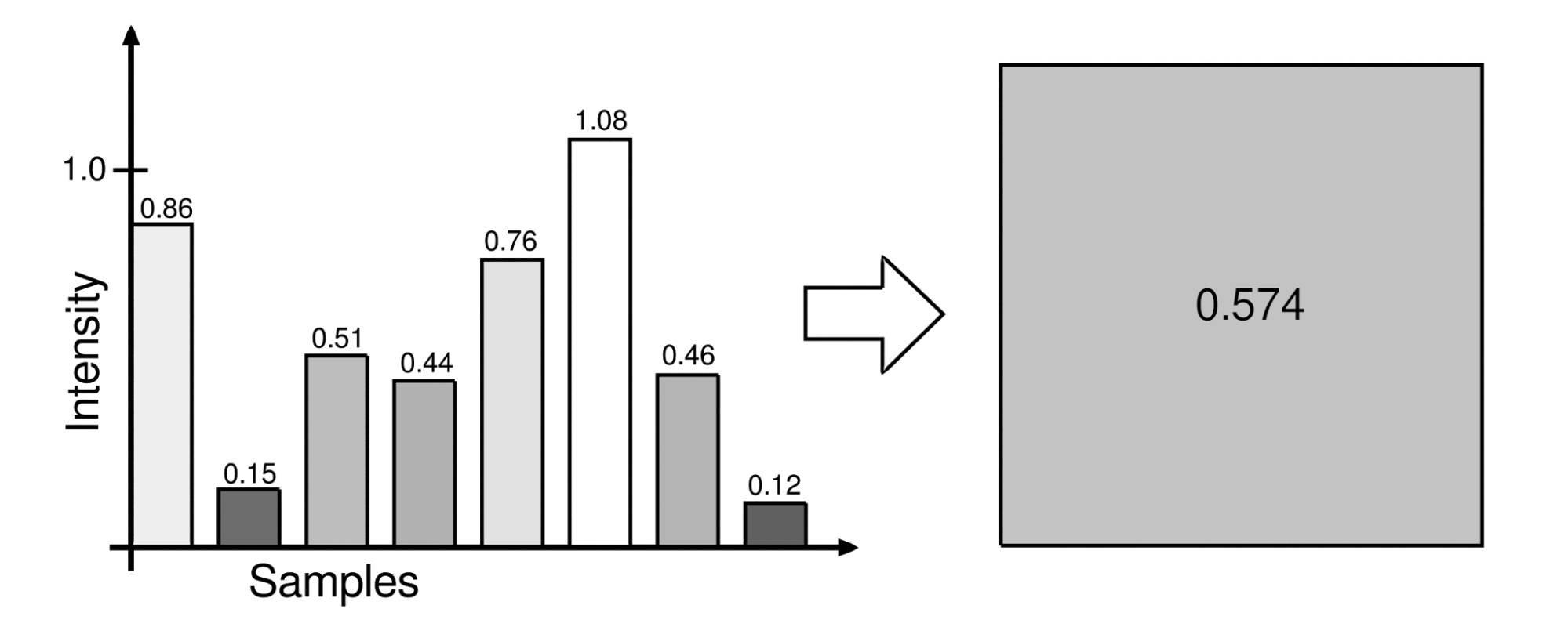
Fig. 1.13) For each pixel, the mean intensity of all samples is used for the final value.
Determining the New Direction of a Ray Hitting a Surface
Fig. 1.11 might look like the path was well-defined, but it illustrates only one of many paths a ray can take. Cycles randomly decides which shader to sample when there are multiple ones in a material. But in many cases there is also a random factor for the direction the ray will take when bouncing. Almost all shaders have an included component that tells Cycles what the chances are for a ray to travel in a specific direction after hitting the surface. Cycles will then randomly pick a possible direction. Directions that are more likely will be picked more often than directions that are less likely. This process is called sampling the shader. For a ray bouncing off a diffuse shader, all directions have an equal likelihood. For a rough glossy shader directions closer to the angle of a sharp reflection are more likely than those further away, see fig. 1.14 and 1.15.
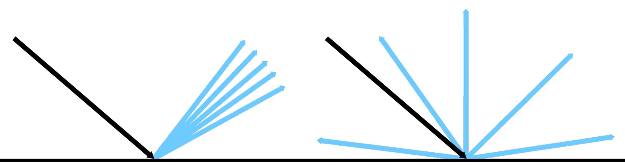
Fig. 1.14) Left: A ray hitting a glossy shader with little roughness and few possible ways for it to continue. Right: A ray hitting a diffuse shader and the possible outcomes. This is the representation we will be using throughout the book for the sake of simplicity.
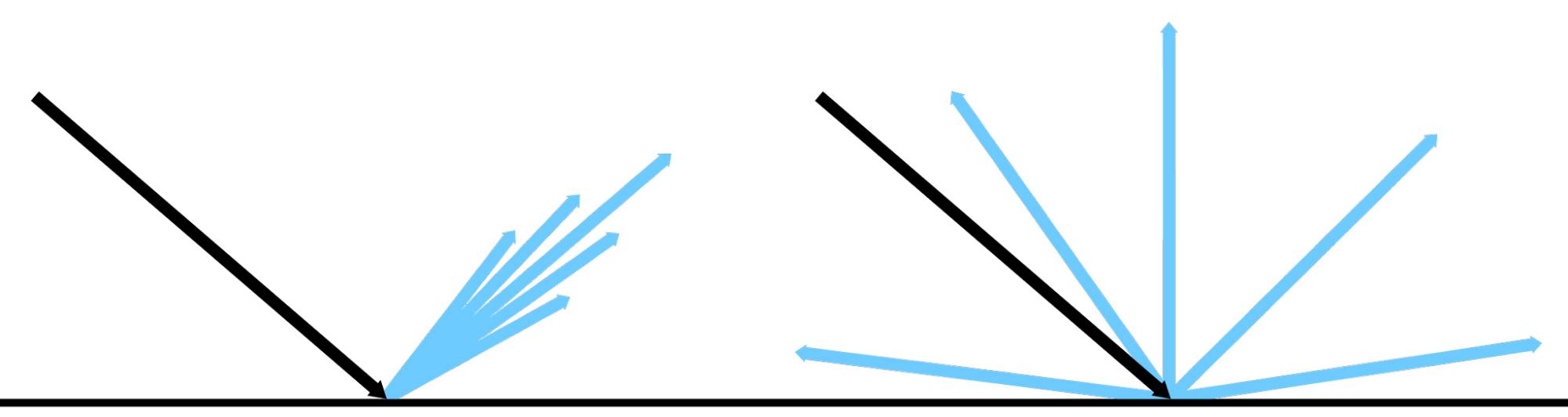
Fig. 1.15) Alternative representation of a ray hitting a diffuse and glossy shader. The length of the arrows denotes the likelihood of a ray continuing in its direction. Left: glossy shader. Directions further away from the angle of reflection are less likely. Right: diffuse shader. All directions have the same likelihood.
With this new information in mind let’s update the example from fig. 1.11. We encounter a big problem: It is actually very unlikely that Cycles finds a path to the light source in the transmission case because the diffuse bounces can head almost anywhere (see fig. 1.16).
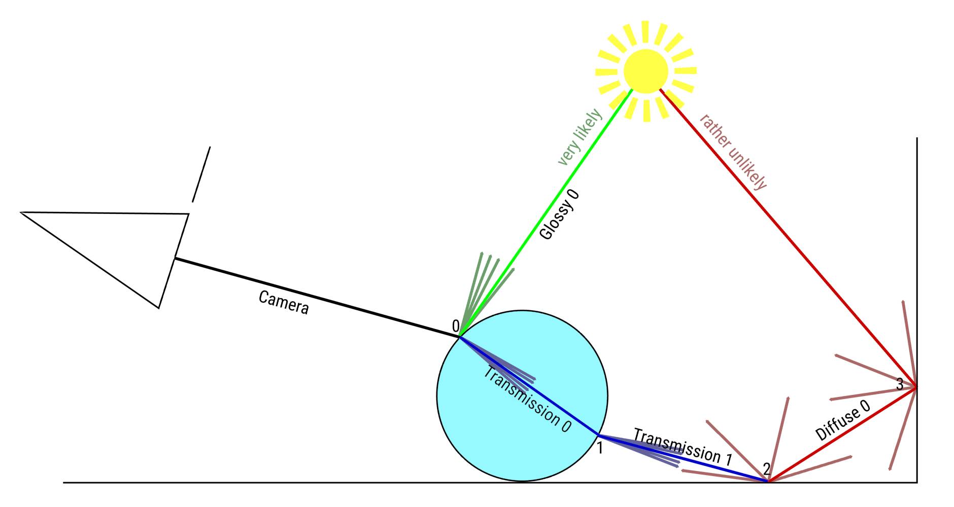
Fig. 1.16) The example from fig. 1.11 with added probabilities for possible directions (dark and desaturated arrows). You see that especially for the last diffuse bounce it is very unlikely that it would actually reach the light source because it could bounce into any other direction as well. For the glossy case at bounce #0 it is much more likely that the ray can hit the light source.
You see that for the second path, there are little chances to reach the light source and thus illuminating that part of the scene. But there is supposed to be light behind that glass sphere. Fortunately Cycles has a smart way to gather lighting information for every bounce: light sampling!
Light Sampling and MIS
This chapter is very technical. You can safely skip it and still achieve great results with Cycles. It also refers to some terms that might be new to you if you are new to Cycles. In that case read the other chapters first. But if you are interested in some theory about path tracing, keep reading. You should also read this chapter if you want to optimize your scenes for less noise and lower render times because it lays out the foundations for understanding how Cycles treats light sources. It may also help you to understand what settings like MIS and properties like is shadow ray are all about.
The process shown in the previous chapters is actually a simplified version of what Cycles does. Actually for each bounce an additional ray is cast. The trick is that Cycles knows where the light sources in your scene are located. So when a ray hits a surface, Cycles will first cast a ray towards a random light source. This process is called light sampling and those rays are called shadow rays . The shadow rays either find their way to the light source or get blocked by geometry. For the former case, the amount of light from that source is stored. Then Cycles will randomly select a shader from the material node tree of the surface. Cycles will then compare the direction of the shadow ray with the possible directions the shader offers (see fig. 1.14 and 1.5) and multiply the light intensity stored for the shadow ray by the probability of bouncing in that direction. This process is called evaluation of the shader. In the next step Cycles will determine where the ray would go next. It will take the stored information of possible directions of the shader (aka the distribution ) and randomly select one. This process is called sampling the shader. The ray will then continue into the new direction.
So what is the difference between sampling and evaluating and shader? Sampling can be described as picking a random direction from the possible directions a shader offers and is used to find a new direction when a ray bounces.
Evaluation means that you are already looking into a specific direction, like in the case of shadow rays, and ask the shader how likely this direction would be if a ray was bouncing off it.
Fig. 1.17 shows what will happen when a ray hits a surface and a light source is in the scene. Cycles will then cast a shadow ray toward that light source.
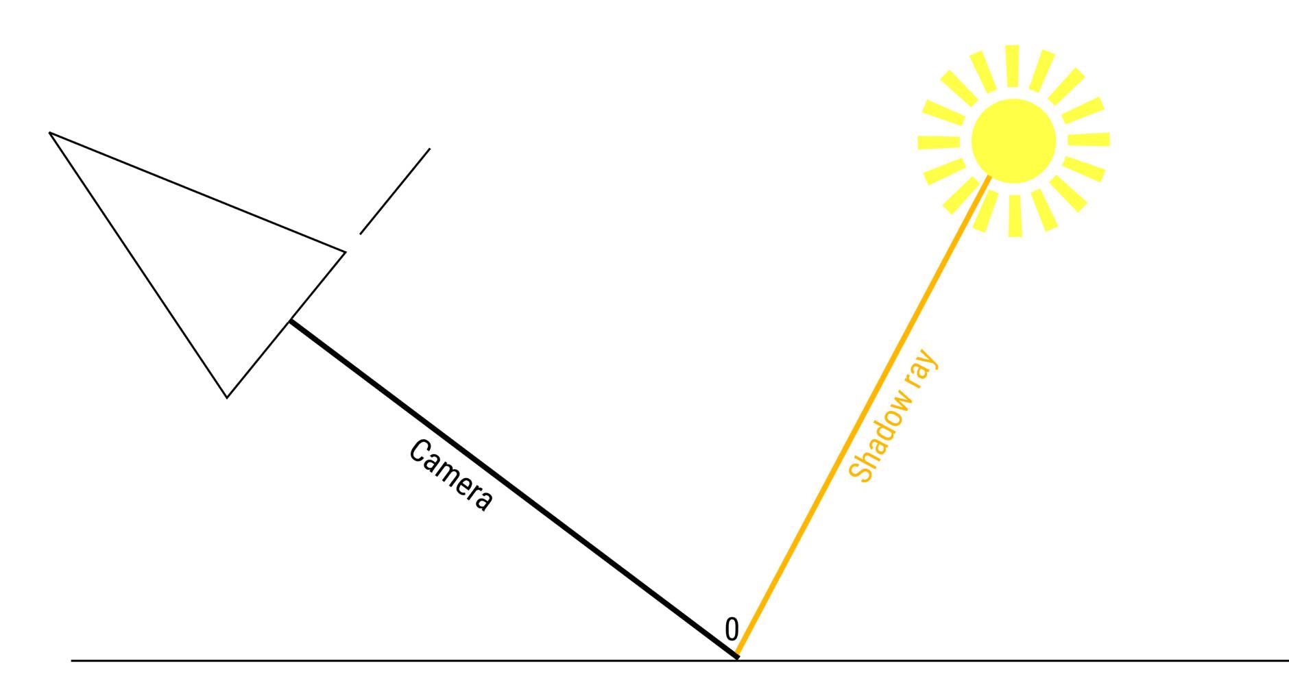
Fig. 1.17) A ray hits a surface. Cycles will first cast a shadow ray towards a random light source.
Cycles then takes a look at the surface, let’s consider a diffuse one for this example. It will then weight the light contribution according to the likelihood of the direction of the shadow ray from the shaders perspective. This process is the aforementioned evaluation of the shader with the direction of the shadow ray, see fig. 1.18.
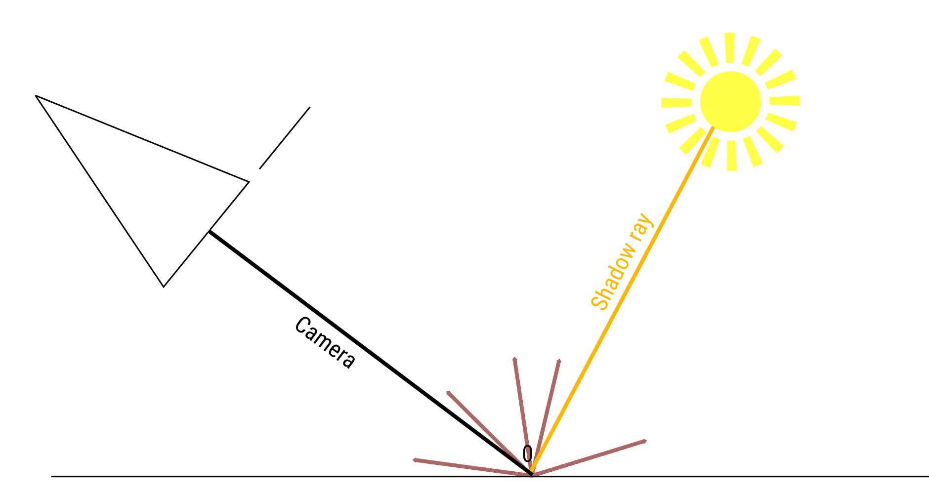
Fig. 1.18) After the shadow ray found the light source, the shader gets evaluated so the contribution of the shadow ray can be weighted by the likelihood of it reaching the light source if it was a regular ray. In the case of a diffuse shader, the likelihood is the same for all directions ( desaturated red arrows ).
After that, Cycles will determine what direction the regular ray will take next by picking a random one out of the direction the shader is offering. That direction might be far away from the light source, but thanks to the shadow ray the bounce can still store information about illumination from the light source, see fig. 1.19.
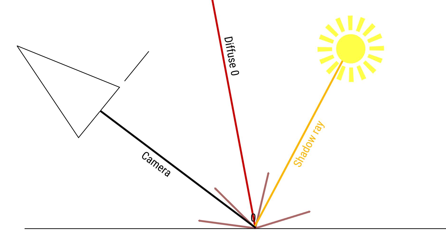
Fig. 1.19) After the shadow ray is cast and the shader evaluated, the new direction for the ray is determined by picking a random direction out of the possible ones the shader is offering ( desaturated red arrows ). This process is called sampling the shader . Even when it chooses a direction where it misses the light source, Cycles can still store illumination information for the bounce thanks to the shadow ray.
Sampling lights using shadow rays is a nice way to reduce noise in a scene because for almost every sampling point information about the illumination from light sources can be gathered. But shadow rays are not infallible. There are some cases where they cannot contribute anything. The first one is, when they are blocked by geometry, because any non-emissive surface, no matter if it is diffuse, glass, glossy or anything else, will block it (with the exception of transparent shaders, which allow shadow rays to continue). That is also where the name shadow ray originates. Because if they are blocked, there will be shadows (see fig. 1.20).
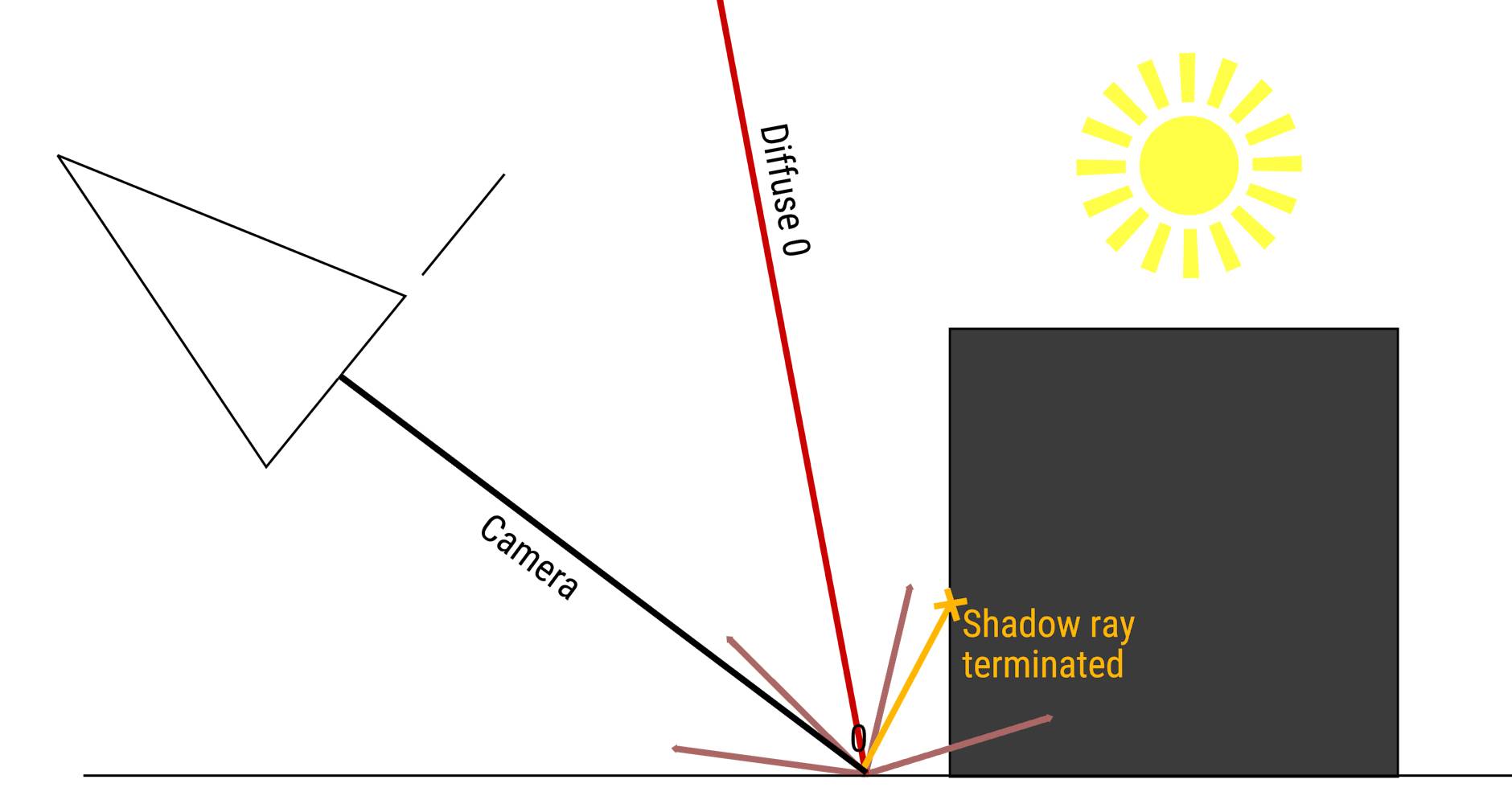
Fig. 1.20) Shadow rays terminate when they hit a non-light surface. That is why they are called shadow rays, because areas where a light source can not be reached will be in shadow.
There is another situation where shadow rays will not be able to contribute lighting information: When the shader of the surface is evaluated after the shadow ray was cast and it tells the shadow ray that the direction it went in is not a direction the shader would allow for regular rays. In that case the lighting information of the shadow ray will be weighted with zero, thus not contributing any lighting information. One example where this can happen is glossy shaders with only little roughness, see fig. 1.21).
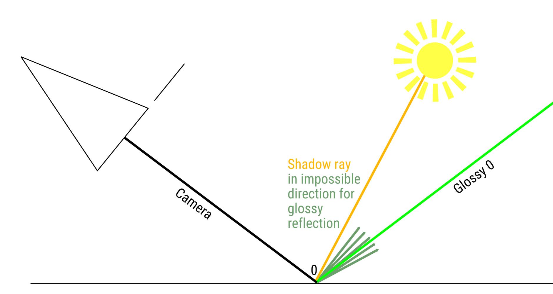
Fig. 1.21) Visualization of the wasted shadow ray problem. The shadow ray is successful in finding a light source. But when the shader is evaluated ( dark green arrows ), its light contribution is weighted zero, because it is outside of the possible directions the glossy shader offers.
What if another light source was in reach of the regular ray, ie. in reach of the possible directions the shader offers? Since Cycles fires shadow rays towards random light sources, there is of course a chance that another light source would have been in reach for the shadow ray, so Cycles simply picked the wrong one.
Since Cycles fires lots and lots of rays, the right one would be chosen at some point. So the wasted shadow ray problem is mostly a problem of wasting processing resources.
It can become a real big problem in case of indirect reflections, aka reflective caustics. See fig. 1.25 for a more detailed explanation.
What happens if a material has multiple shaders in it? Since shadow rays are cast before the shader is evaluated, a shadow ray gets cast and then the regular ray will decide which of the shaders to follow, see fig. 1.22.
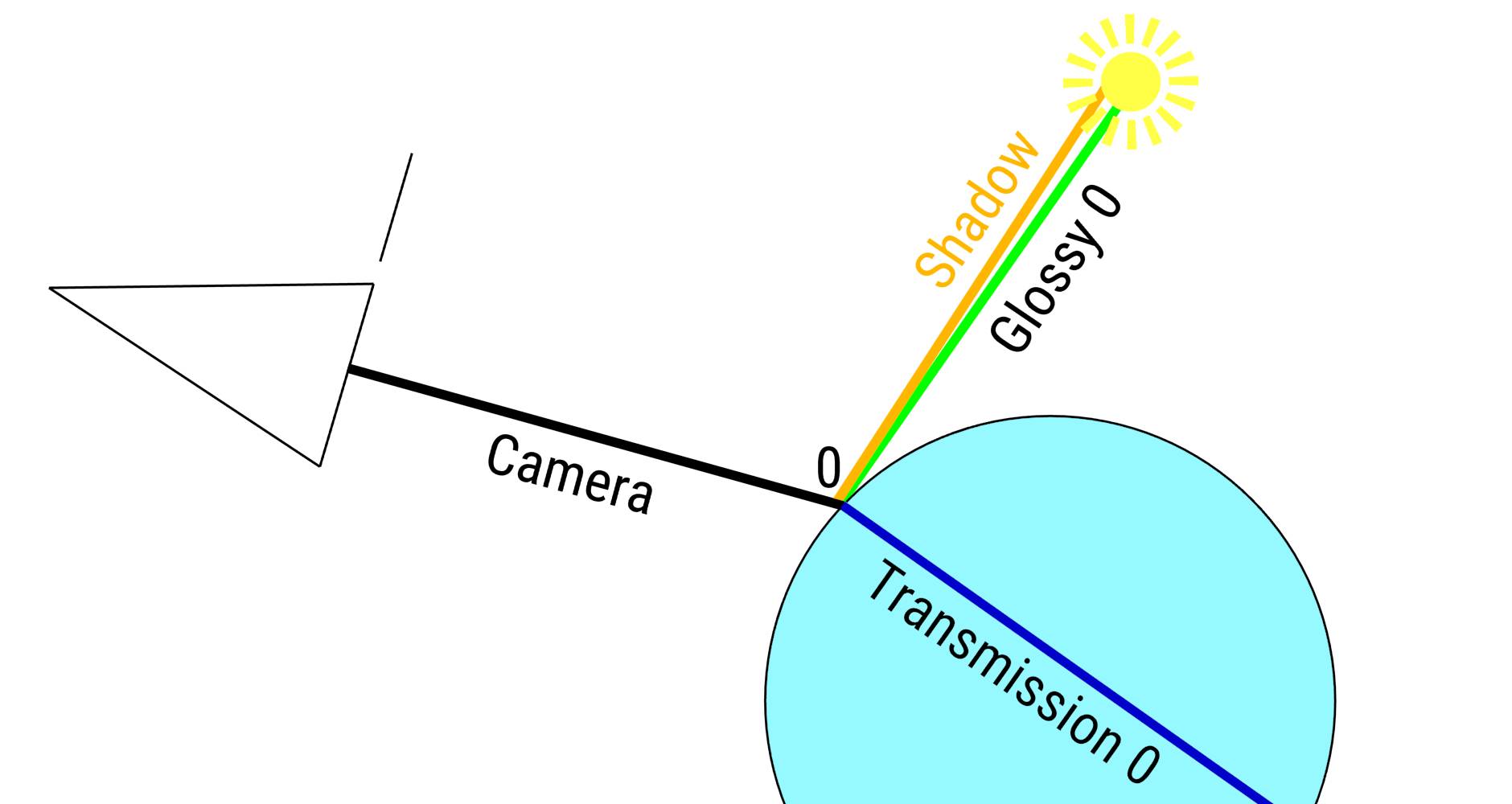
Fig. 1.22) When a ray hits a surface with multiple shaders in its material ( like glass for example ), a shadow ray gets cast first, then Cycles decides which shader to follow. In this example, two alternate paths are shown and the one shadow ray. Note that shadow rays aim at a random point on the light source’s surface, not just the center.
Let’s revisit the scene from fig. 1.11 with added shadow rays:
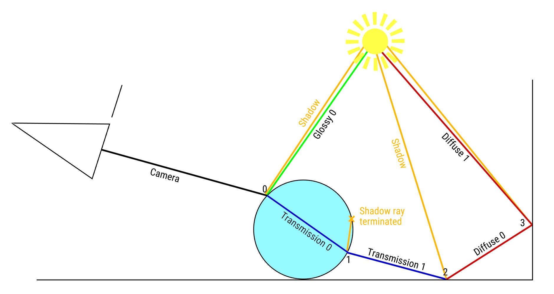
Fig. 1.23) The example from above revisited but with added shadow rays. For every bounce Cycles will send a shadow ray towards a random light source. Shadow rays get blocked by any geometry, though. Even if it is glass (bounce #1).
Unless the shadow ray gets blocked by geometry like in fig. 1.23 bounce #1, Cycles can store the light contribution of the source for each point. Take a look at the last diffuse bounce (#3). It is actually very unlikely that this bounce would reach the light source because diffuse bounces are just random, and it is likely to hit the ground or the back of the sphere next. So let’s make sure that it does not reach the light at all by lowering the maximum bounces to 2 in the next example, which will also show you that shadow rays are not cast on terminating bounces, see fig. 1.24.
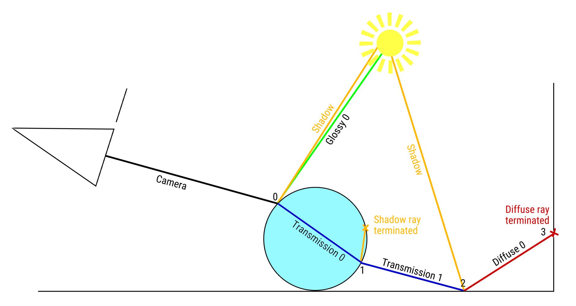
Fig. 1.24) In this example the ray gets terminated on the transmission route before it can reach a light source, because the maximum number of bounces (2) is exceeded. But thanks to light sampling aka shadow rays, Cycles can still get some light information for this pixel from the shadow rays that found their way to the light source at bounce #0 and bounce #2. Shadow rays do not get cast at a terminating bounce (#3).
The reason why Cycles is casting shadow rays is to make images clear up a lot faster. Even for rays that do not hit a light source Cycles can get light information this way (see fig. 1.24), which will result in less noise in your renders.
Fig. 1.24 shows two shadow rays finding the light source for the transmission case. But only one of them will contribute actual lighting information (bounce #2), the other one will contribute nothing (bounce #0). At bounce #0 we can see a shadow ray finding the light source, but the blue path would not allow any ray to travel into this direction. Therefore only the shadow ray at bounce #2 contributes light information for the transmission case, see fig. 1.25.
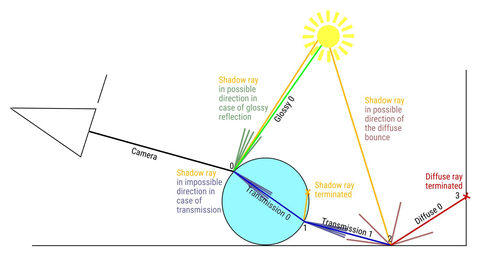
Fig. 1.25) The example from fig. 1.24 extended by the illustration of the directions a path could potentially take. Before the ray decides to either reflect off or enter the surface at bounce #0 , a shadow ray is cast towards the light source. For the reflective case ( green ) that results in a light contribution because the angle of the shadow ray is well inside the limit the glossy shader imposes in this case ( dark green arrows ). But if the ray decides to enter the glass object, the same shadow ray will not illuminate the bounce, because no ray going through the glass ( violet arrows ) could possibly reach that light source. So actually only bounce #2 will contribute light because the shadow ray has a direction that could be taken by the actual (diffuse) ray as well ( desaturated red arrows ).
You can tell from fig. 1.25 that sharp glossy reflection and refractions reduce the chances that a shadow ray can actually contribute light to a bounce even if it finds a way to the light source. That is the reason why refractive and reflective caustics are usually a source for noise in the scene, because shadow rays have a hard time to do their work with that kind of shaders . For refractive materials it’s even worse due to shadow rays terminating when cast from inside a glass object (bounce #1).
Shadow rays can be cast towards lamps as well as objects with an emission shader in their material, if they have Multiple Importance Sample (MIS) enabled. In that case Cycles will also store the location of the emissive objects with MIS and sample them just like lamps. By default MIS is turned on for all objects so you do not need to worry about that. MIS can also be used on the environment, .
Lamps also have an MIS option, but there the situation is reversed. By default MIS is turned on and they are visible for all ray types. If you turn MIS off on a lamp, they will only be visible to shadow rays, meaning a regular ray will only terminate on emissive surfaces but not when hitting a lamp. So lamps will not be visible in caustics and sharp glossy reflections in that case.

