Now we are going to explore Mathematica, an awesome programming language that is used in engineering, mathematics, science, and more. It can work with images, sound, maps, and 3D graphs, as well as access massive sets of data of the internet – and work with GPIO! This is going to be a quick introduction to some of its capabilities.
Basics
To start off with, you need to go to the GUI, and if you aren’t there, then click Ctl-Alt-F2. Once inside, go to Programming … Mathematica.
You’ll see a screen that says Untitled – Wolfram Mathematica. This is called the notebook editor, where you will type in the Mathematica commands you want the computer to run. To start, we’re going to create another Hello, World type of program. It’s really easy!
First, click inside the notebook editor and then type this command: Print[“Hello, World!”]
Press Shift-Enter to run the command. What you should see on the screen, below the command you typed in, is …
Hello, World
You have now written your first Mathematica program!
Access to Online Data
One of the features that makes Mathematica different is its special features, including its ability to quickly access online data. We can write a one-line program that will pull up a street map that shows your current location (but only if you are connected to the Internet). Here is what you need to type in – be careful with punctuation and capitalization:
GeoGraphics[GeoMarker[],GeoRange->Quantity[1,”Miles”]]
Now press Shift-Enter to run the command. If you are connected to the internet, you will see a street map on your screen.
Mathematica can access customized weather data for your area, too. Try this slightly longer program:
loc=$GeoLocation;
Print[“Weather Report for “, Now];
Print[“Current Temperature: “, WeatherData[loc[[1]],”Temperature”]];
Print[“Current Wind Speed: “, WeatherData[loc[[1]],”WindSpeed”]];
Press Shift-Enter to run these commands. You should see something like this on your screen:
Weather Report for Wed 3 May 2016 10:05:23
Current Temperature: 26.9 C
Current Wind Speed: 1.2 km/h
What happened when you ran that code is as follows: Mathematica went online to retrieve the data from weather stations near your location (indicated by the keyword GeoLocation) and then displayed what it found for temperature and wind speed at the current time (indicated by the keyword Now). You can also check humidity, pressure, dew point, conditions, etc.
Let’s look at the program line by line to see how it works.
loc=$GeoLocation;
This command tells Mathematica to determine your location in Geodesic coordinates. If you want to see what those Geodesic coordinates look like take the semicolon ; off the end of the line code and run the instructions again. The semicolon, called a suppression operator, keeps intermediate numbers and results from appearing on the screen (suppresses them).
As with Python, Mathematica set aside a spot in memory to be associated with the variable loc, then stores the Geodesic coordinates for your location in it. That way it doesn’t have to keep looking the coordinates up – it can just retrieve them from the variable loc.
Print[“Weather Report for “, Now];
Print is used to display something to the screen. Everything between the outermost square brackets is telling Print what to display. Everything in double quotes will appear exactly as it is written. The keyword Now retrieves the exact time the command is issued – date, year, hour, minute, and second. Let’s go to the next line.
Print[“Current Temperature: “, WeatherData[loc[[1]],”Temperature”]];
The WeatherData command tells Mathematica to look up the weather data for the location that was stored in loc. Temperature tells the WeatherData command that you want it to retrieve the current temperature. The reason that loc is written loc[[1]] is because when you retrieved your position and stored it in loc, Mathematica retrieved something like this:
GeoPosition[{32.51, -94.8}]
The WeatherData command just needs this part: {32.51, -94.8}
If you try typing in loc[[1]] you will see that it extracted just the part we need for the Weather Data command.
GPIO
Mathematica can also be used to read and write to pins on the GPIO board. First, though, you need to access Mathematica as a superuser, just like you had to do for Python. Open the LXterminal and type this: sudo mathematica
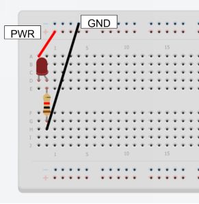
On your breadboard, use the same circuit as we did for the Python example. We are going to write a program to do the same thing, but this time it will be in Mathematica. We are also going to use the same pins, but in Mathematica we are going to refer to the output pin by its GPIO#.
In Mathematica, type these commands exactly as they appear:
DeviceWrite[“GPIO”,4->1]
AbsoluteTiming[Pause[5]];
DeviceWrite[“GPIO”,4->0]
Click Shift-Enter to run your program, and you should see your LED light up for 5 seconds, then turn off. Let’s see how this code works by studying each command.
DeviceWrite[“GPIO”,4->1] tells Mathematica to set GPIO#4 (pin 7) to 1, just as we set it to True in Python. Recall that we when we want to change the level of a pin we write to it, and when we want to check the level of a pin we read from it.
The command AbsoluteTiming[Pause[5]] tells Mathematica to Pause for five seconds, based on absolute time (hence the command AbsoluteTiming) as opposed to CPU clock time.
DeviceWrite[“GPIO”,4->0] tells Mathematica to set GPIO#4 (pin 7) to 0, just as we set it to False in Python.
And that is how easy it is to setup your code in Mathematica! Be sure to look at the online resources that document all the other GPIO commands you can access from Mathematica.
Online Resources:
Mathematica GPIO:
Mathematica Raspberry Pi:
Tweeting from Raspberry Pi:
Getting Started with Mathematica:
Using the Wolfram Language with Raspberry Pi GPIO:


