Chapter 8
Projects and 3D examples
It is best to expand upon the overview of information presented in this book with a collection of examples. Each example will use different parts of the Blender interface to implement a different style of scientific visualization. Example blend files, data files and videos will be provided to better illustrate some of these features.
8.1 3D scatter plot
A 3D scatter plot can be useful in showing trends in multiple parameters or the locations of objects in 3D space. In this project stars from the Hipparcos project will be displayed in 3D []. The concepts used will be:
- Reading in formatted data with the Blender Python API.
- Setting up a Cartesian grid.
- Moving the camera around the dataset.
The following steps will set up this visualization.
- Add a plane with Add → Mesh → Plane. Scale the plane with the S key and press TAB to enter Mesh Edit mode. Subdivide the plane five times and press TAB one more time to again return to Object mode.
- Add a material to the plane mesh on the Properties panel and set the type to ‘Wire’. Choose a color that contrasts well with the background—blue on black usually works well.
- Set the World tab background horizon color on the Properties panel to black.
- Add a simple mesh with Add → Mesh → Circle. Press TAB to enter Mesh Edit mode, SHIFT select all but one of the vertices and press X to remove them. Press TAB one more time to go back to Object mode.
We then import the Hipparcos catalog with the following Python script:
import bpy
import math
import bmesh
import csv
obj = bpy.data.objects['Circle']
if obj.mode == 'EDIT':
bm = bmesh.from_edit_mesh(obj.data)
for v in bm.verts:
if v.select:
print(v.co)
else:
print("Object is not in edit mode")
bm = bmesh.from_edit_mesh(obj.data)
#Read in Hipparcos data
filename = 'hygxyz.csv'
fields = ['StarID','HIP','HD','HR','Gliese','BayerFlamsteed',
'ProperName','RA','Dec','Distance','PMRA','PMDec','RV','Mag',
'AbsMag','Spectrum','ColorIndex','X','Y','Z','VX','VY','VZ']
reader = csv.DictReader(open(filename), fields, delimiter=',')
dicts = []
#Skip first header line
next(reader)
for row in reader:
dicts.append(row)
#Add in vertex elements with XYZ coordinates at each row
for row in dicts:
xpos = float(row['X'])/100.0
ypos = float(row['Y'])/100.0
zpos = float(row['Z'])/100.0
bm.verts.new((xpos,ypos,zpos))
bmesh.update_edit_mesh(obj.data)
- The data should load quickly. We can now add a material to the Hipparcos data points.
- Select the data points and click the Materials tab on the Properties panel.
- Select ‘Halo’ and change the size value to 0.005 and hardness value to 100. A white or light yellow color can be used to color the points.
We can now use the default camera object to point at an empty object as in section .
- Add an empty object with Add → Empty → Plain Axes for the camera to track (figure ).
- Right-click to choose the camera object and set the position and rotation values on the Transform toolbar to zero.
- Click the Constraints tab on the right-hand side Properties panel.
- Choose ‘Track To’ and select the target as ‘Empty’.
- Select ‘To’ as –Z and ‘Up’ as Y. This will correctly orient the upward and normal directions when looking through the camera field of view.
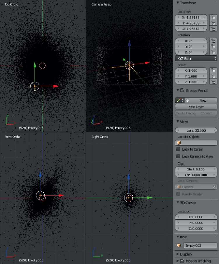
Figure 8.1. The set-up for an empty tracking object. The camera will point to this object during the fly through of the Hipparcos catalog.
Animate the visualization by keyframing the camera.
- This animation will be 20 s long at 30 frames per second. Therefore set the number of frames to 600 and set the current frame to 1.
- Right-click to select the camera and press the I key to keyframe the position and rotation of the camera.
- On the Animation toolbar, set the current frame to 600. Move the camera in the 3D view port to a different location and orientation.
- Keyframe the camera position and rotation one final time with the I key.
The visualization can now be exported in a 1080p HD video.
- On the Render tab in the Properties panel select HDTV 1080p and set the frame rate to 30 frames per second.
- Set the output to AVI JPEG, quality 100 percent, and specify a unique filename. Click the ‘Animation’ button at the top of the tab to render the visualization. A frame from the final animation is shown in figure .
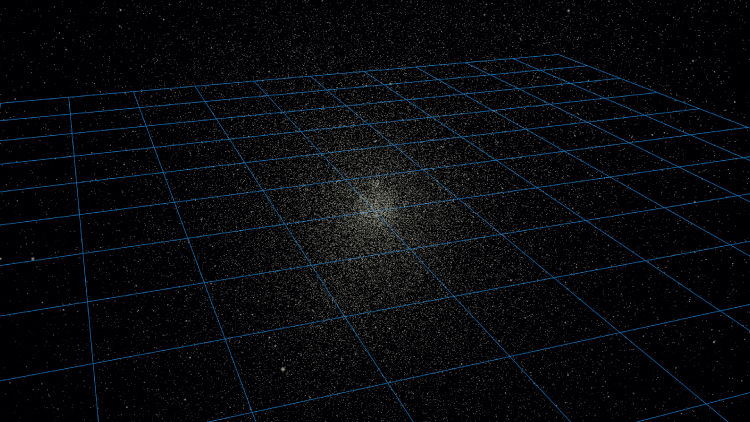
Figure 8.2. A 3D rendering of the Hipparcos catalog, utilizing a halo material, a subdivided grid and camera tracking.
8.2 N-body simulation
For this example we will provide the reader with N-body data from a galaxy collision simulation. The idea is to expand upon the initial scatter plot example by putting the N-body points into shape keys to improve performance and then iterate over each snapshot to complete the animation. The concepts used will be:
- Reading in multiple files of formatted data with the Blender Python API.
- Setting up a Cartesian grid.
- Associating each temporal snapshot with a shape key.
- Adding halo materials to the data points.
- Moving the camera to track to the centroid of a galaxy until a specified time during the galaxy collision.
This example of a galaxy simulation was generated with GADGET-2 [], an extremely useful N-body and smoothed particle hydrodynamics package for astrophysics. Its capabilities range from large scale structure cosmology simulations to galaxy collisions. The simulation in this example is run for approximately 1100 time steps for a total run time of two billion years. Each large spiral disk galaxy has 10 000 disk particles and 20 000 halo particles with Milky Way scale lengths and masses (2.1 kiloparsecs and 109 solar masses). The particle position data are shown as a single vertex with a halo material. Each snapshot is keyframed as a camera object is flown along a Bézier curve. A frame from the animation is shown in figure .
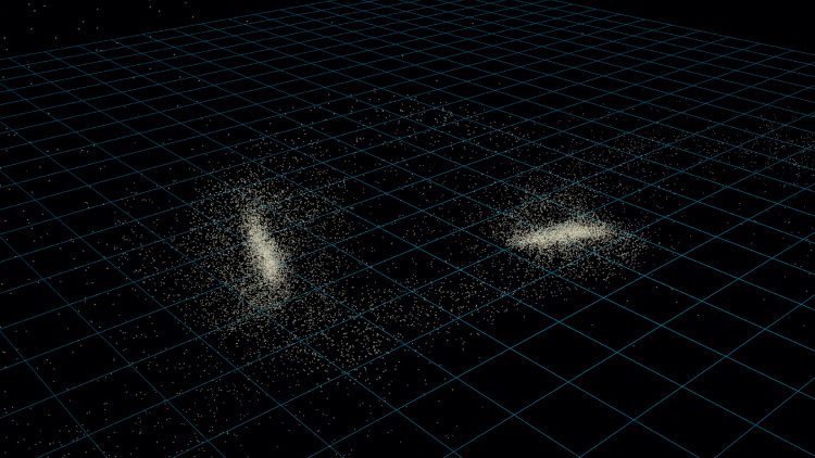
Figure 8.3. A 3D rendering of an N-body simulation showing a collision between two galaxies.
The ASCII snapshot files produced by the simulation are in the following simple X, Y, Z comma-separated-value format:
-44.4367,-44.1049,-0.539139
-94.6014,-74.8028,-0.5839
-70.9394,-77.0528,-0.357556
-58.1572,-57.4876,-0.917166
-63.3899,-61.3828,-0.793917
...
First a shape key needs to be created in the script with (for this simulation) 20 000 vertex points:
import bpy
import bmesh
#Switch to object mode
bpy.ops.object.mode_set(mode = 'OBJECT')
#Create initial Basis Shape Key
bpy.ops.object.shape_key_add()
#Create initial Shape Key
bpy.ops.object.mode_set(mode = 'OBJECT')
bpy.ops.object.shape_key_add()
bpy.data.shape_keys[0].key_blocks["Key 1"].name = 'Key 1'
bpy.data.shape_keys[0].key_blocks["Key 1"].value = 1
bpy.data.shape_keys[0].key_blocks["Key 1"].
keyframe_insert ("value", frame=0)
The snapshot data files are then read in using the csv and glob Python module. The vertices are added to a single vertex circle object just like the mesh created in the 3D scatter plot example.
import glob
import csv
import bpy
import bmesh
files = glob.glob('*.txt')
files.sort()
for f in files:
fields = ['X', 'Y', 'Z']
csvin = csv.DictReader(open(f), fields, delimiter = ',')
data = [row for row in csvin]
dicts = data
obj = bpy.data.objects['Circle']
mesh = obj.data
bm = bmesh.from_edit_mesh(obj.data)
rowcount = 0
for i in range(0,len(bm.verts)-1):
try:
bm.verts[i].co.x = float(dicts[rowcount]['X'])/10.0
bm.verts[i].co.y = float(dicts[rowcount]['Y'])/10.0
bm.verts[i].co.z = float(dicts[rowcount]['Z'])/10.0
rowcount += 1
bmesh.update_edit_mesh(obj.data)
except:
pass
Add in the keyframes for each shape key:
#Key a single frame per data file
for j in range(1, frames+1):
for keyname in bpy.data.shape_keys[0].key_blocks.keys():
if keyname != os.path.basename(files[framecount-1]):
bpy.data.shape_keys[0].key_blocks[keyname].value = 0
bpy.data.shape_keys[0].key_blocks[keyname].
keyframe_insert("value", frame = framecount)
framecount += 1
We now change the vertices to have a material texture of a small Gaussian sphere.
- With the circle object selected, click on the Materials tab in the Properties panel to create a new material with the ‘Halo’ option.
- Change the halo size to 0.05.
- Change the hardness to 100.
- Modify the desired halo color to your liking.
Since both galaxies are moving, we will keyframe an empty object to track the centroid of one galaxy before the collision. As the collision evolves the empty object will slow to a stationary position (figure ). The camera object will also move and track the empty object during the entire animation.
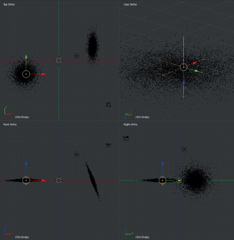
Figure 8.4. An empty object is placed at the centroid of one of the galaxies and keyframed to move during the camera tracking.
- Add an empty object with Add → Empty → Plain Axes for the camera to point toward.
- With the current frame set to zero, place the empty object near the center of a galaxy and keyframe the position with the I key.
- Play the animation through the first part of the collision and then stop. Move the empty object to a new position near the collision centroid and add another keyframe.
- Right-click to choose the camera object and set the position and rotation values on the Transform toolbar to zero.
- Click the Constraints tab on the right-hand side Properties panel.
- Choose ‘Track To’ and select the target as ‘Empty’.
- Select ‘To’ as –Z and ‘Up’ as Y. This will correctly orient the upward and normal directions when looking through the camera field of view.
Snapshots and different camera views from the final animations are shown in figure .
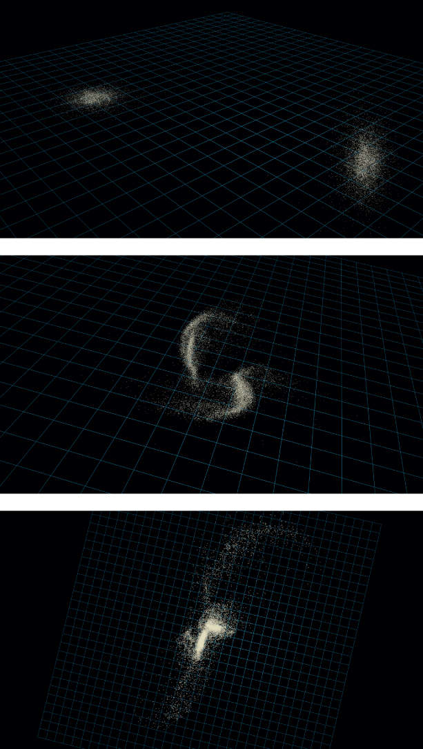
Figure 8.5. Frames from an N-body galaxy collision simulation.
8.3 Magnetic fields
In this project we will produce a 3D visualization of the magnetic potential for a loop of electric current. The concepts used will be:
- Evaluating the appropriate equations in Python for the magnetic potential.
- Add a model for the current loop using extrusion.
- Plot the contours using vertex editing mode.
- Rotate the contours due the azimuthal symmetry of the equation.
- Add a colored wire material for the potential contours.
From classical electrodynamics we know that the current density J has an azimuthal component in a ring of radius a. Reviewing these basic equations we have []:

The solution for the vector potential is written as:

Due to the symmetry of the configuration, we can write the azimuthal component  as:
as:

where K(k) and E(k) are complete elliptic integrals. The solution can be expanded in the following approximation:

We will evaluate this expression, compute the contours and use vertex editing mode to draw the contours. Because the scenario is azimuthally symmetric, we can use the Blender spin tool to rotate the magnetic potential contours about the Z-axis. Finally, we will add the current loop and animate the visualization. The data from are generated and read in via the following Blender Python script:
import pickle
import numpy
import bpy
import bmesh
import csv
obj = bpy.data.objects['MagneticField']
bpy.ops.object.mode_set(mode = 'EDIT')
bm = bmesh.from_edit_mesh(obj.data)
#Read in contour data
filename = 'magnetic.txt'
fields = ['X', 'Y']
csvin = csv.reader(open(filename))
data = [row for row in csvin]
dicts = []
for row in data:
datarow = map(float,row[0].split())
rowdict = dict(zip(fields, datarow))
dicts.append(rowdict)
for row in dicts:
try:
xpos = row['X']
ypos = row['Y']
bm.verts.new((xpos,ypos,0.0))
bmesh.update_edit_mesh(obj.data)
#Note that the minus 2 is the number of points to connect
bm.edges.new((bm.verts[i] for i in range(-2,0)))
except:
print("Skipping")
bmesh.update_edit_mesh(obj.data)
bpy.ops.object.mode_set(mode='OBJECT')
The ring of current is created using the extrude tool.
- Add a mesh with Add → Mesh → Circle.
- Enter Mesh Edit mode with the TAB key.
- Extrude the vertices with the E key followed by a single mouse click.
- Scale the new set of vertices with the S key and then return to Object mode with the TAB key.
- On the Transform toolbar set the dimensions to 1.5 units in size to match the values used in the model.
- Color the current loop with a blue material.
Due to azimuthal symmetry, the contours can be extended via the spin tool (figure ).
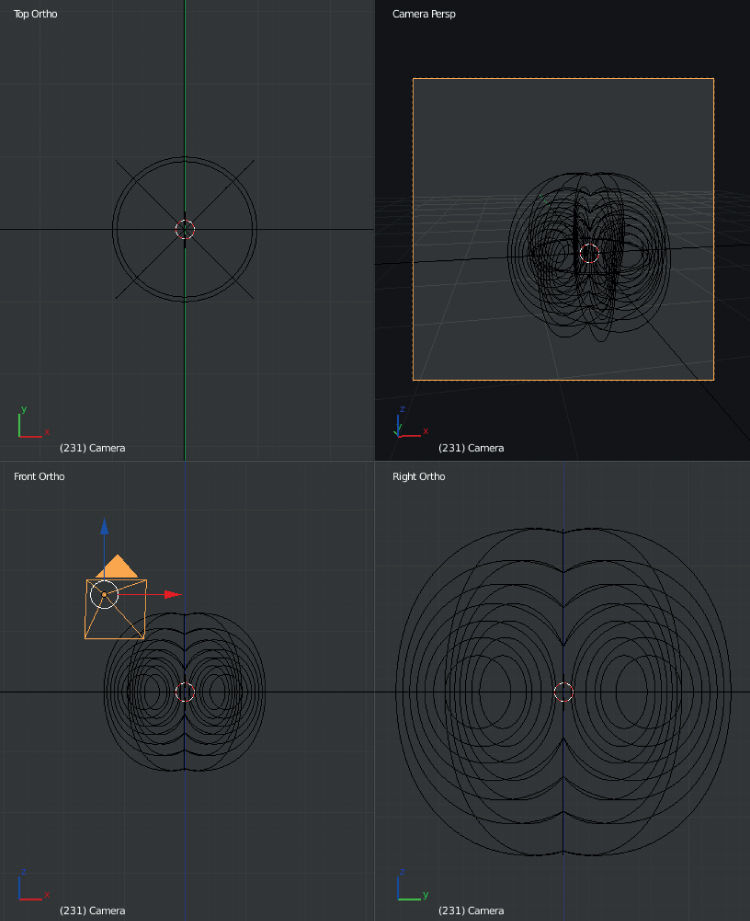
Figure 8.6. Quad view along each axis along with the camera view for the magnetic potential.
- Select the magnetic potential contour mesh.
- Enter Mesh Edit mode with the TAB key.
- Choose ‘Spin’ from the Mesh toolbar on the left-hand side.
- Set the steps to 6, angle to 360, center to zero and Z-axis to 1.0. Check the duplicate box and this will create a set of azimuthally symmetric contours.
- Exit Mesh Edit mode with the TAB key and color the potential contours loop with a red material (figure ).
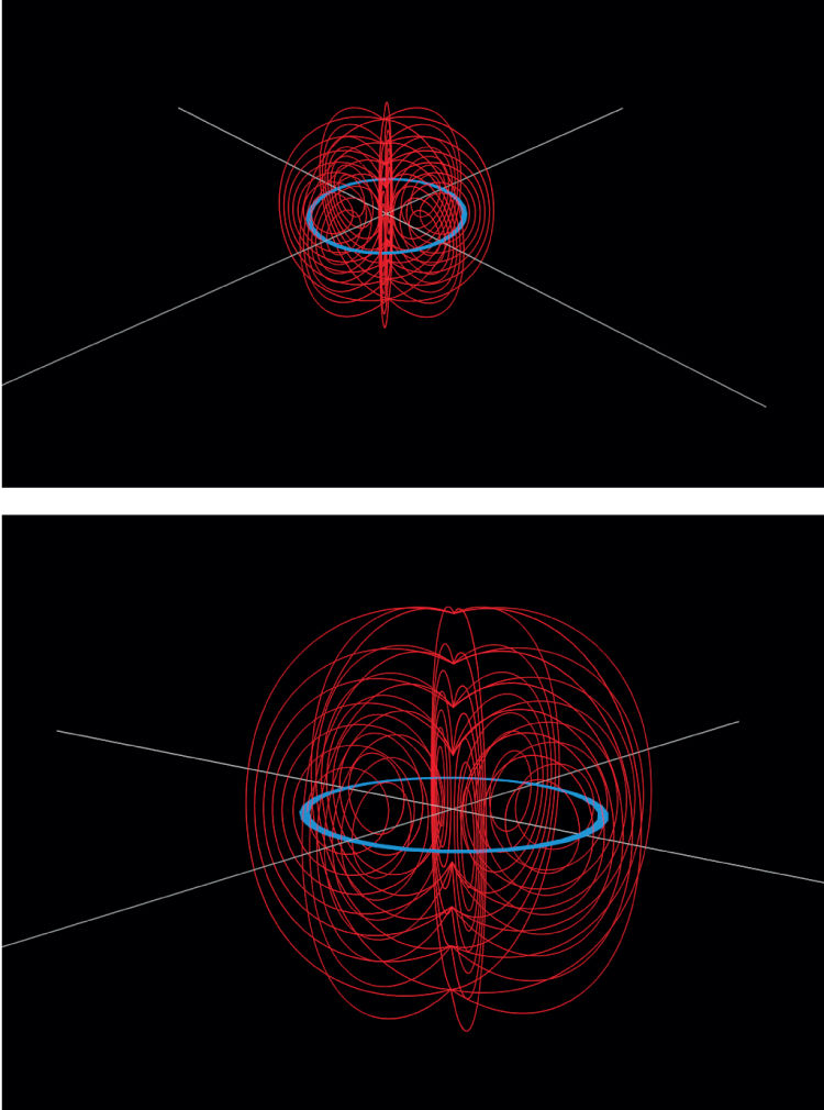
Figure 8.7. A 3D rendering of the magnetic potential for a current loop.
8.4 Lagrangian equilibrium and zero-velocity curves
We can compute and map the Lagrangian equilibrium points and zero-velocity curves for a two mass system. This project will use the following concepts:
- Render the curves as 3D surfaces of revolution.
- Introduce the transparency properties for Blender materials.
- Duplicate mesh models to calculated positions.
The formulation considered here is outlined in chapter of Solar System Dynamics []. We consider two masses in circular orbits of masses m1 and m2 about a common center of mass at the origin O. The sum of the masses and the constant separation between them are both unity. q is the ratio of the masses and we define:


The location of the triangular Lagrangian points L4 and L5 can be solved for:


The collinear Lagrangian equilibrium points are derived as:


We can further refine these collinear Lagrangian points by using the Newton–Rhapson method to solve for the vectors r1 and r2. These examples are included at the book website. Next we provide code that solves for these points.
import math
import os
import csv
import numpy as np
from scipy.optimize import fsolve
import numpy as np
from scipy.optimize import newton
import matplotlib.pyplot as plt
def dPotential1(r, *mus):
errflg = 0
#Unpack tuple
mu1, mu2 = mus
T1 = 1. - r
T2 = T1 - 1.0/T1**2
T3 = r - 1.0/r**2
dU = mu1*T2 - mu2*T3 # Equation 3.73
return dU
def dPotential2(r, *mus):
errflg = 0
#Unpack tuple
mu1, mu2 = mus
T1 = 1. + r
T2 = T1 - 1.0/T1**2;
T3 = r - 1.0/r**2;
dU = mu1*T2 + mu2*T3 #Equation 3.85
return dU
def dPotential3(r, *mus):
errflg = 0
#Unpack tuple
mu1, mu2 = mus
T1 = 1. + r
T2 = r - 1.0/r**2
T3 = T1 - 1.0/T1**2
dU = mu1*T2 + mu2*T3 # Equation 3.90
return dU
def Potential(x, *data):
#Unpack tuple
y, z, mu1, mu2, Vref = data
r1 = math.sqrt((x+mu2)**2 + y**2 + z**2)
r2 = math.sqrt((x-mu1)**2 + y**2 + z**2)
T1 = 1.0/r1 + 0.5*r1**2
T2 = 1.0/r2 + 0.5*r2**2
# Equation 3.64 in Murray and Dermott
U = mu1*T1 + mu2*T2 - 0.5*mu1*mu2 - Vref
return U
def Potential2(y, *data):
#Unpack tuple
x, z, mu1, mu2, Vref = data
r1 = math.sqrt((x+mu2)**2 + y**2 + z**2)
r2 = math.sqrt((x-mu1)**2 + y**2 + z**2)
T1 = 1.0/r1 + 0.5*r1**2
T2 = 1.0/r2 + 0.5*r2**2
# Equation 3.64 in Murray and Dermott
U = mu1*T1 + mu2*T2 - 0.5*mu1*mu2 - Vref
return U
#‐‐‐‐‐‐‐‐‐‐‐‐‐‐‐‐‐‐‐‐‐‐‐‐‐‐‐‐‐‐‐‐‐‐‐‐‐‐‐‐‐‐‐‐‐‐‐‐‐‐
# secondary / primary mass: M2/M1 (M1 > M2)
q = 0.2
# Number of points used in contour plot and in Roche Lobe
npts = 251
# Number of contours in contour plot
nc = 75
#Equations are from Solar System Dynamics by Murray and Dermott
# Equation 3.1
mu_bar = q / (1.0 + q)
# Equation 3.2, Location of Mass 1 (primary) is (-mu2, 0, 0)
mu1 = 1.0 - mu_bar
# Equation 3.2, Location of Mass 2 (secondary) is (mu1, 0, 0)
mu2 = mu_bar
#Define the Lagrangian Points
ratio = mu2 / mu1
alpha = (ratio/3.0)**(1.0/3.0) # Equation 3.75
L1_r2 = alpha - alpha**2/3.0 - alpha**3/9.0 - 23.0*alpha**4/81.0
L1_y = 0.0 # Equation 3.83
L2_r2 = alpha + alpha**2/3.0 - alpha**3/9.0 - 31.0*alpha**4/81.0
L2_y = 0.0 # Equation 3.88
# Equation 3.93
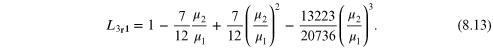
beta = -7.0*ratio/12.0 + 7.0*ratio**2/12.0 - 13223.0*ratio**3/20736.0
L3_r1 = 1.0 + beta
L3_y = 0.0 # Equation above 3.92
L4_x = 0.5 - mu2
L4_y = +sqrt(3.0)/2.0 # Equation 3.71
L5_x = 0.5 - mu2
L5_y = -sqrt(3.0)/2.0 # Equation 3.71
# L4 and L5 are done.
# Corrections to L1, L2, and L3...
L1_r2 = newton(dPotential1, L1_r2, args=(mu1,mu2))
L1_r1 = 1.0 - L1_r2 # Equation 3.72
L1_x = L1_r1 - mu2 # Equation 3.72
L2_r2 = newton(dPotential2, L2_r2, args=(mu1, mu2))
L2_r1 = 1.0 + L2_r2 # Equation 3.84
L2_x = L2_r1 - mu2 # Equation 3.84
L3_r1 = newton(dPotential3, L3_r1, args=(mu1, mu2))
L3_r2 = 1.0 + L3_r1 # Equation 3.89
L3_x = -L3_r1 - mu2 # Equation 3.89
# Now, calculate the Roche Lobe around both stars
# Potentials at L1, L2, and L3
L1_U = Potential(L1_x, 0.0, 0.0, mu1, mu2, 0.0)
L2_U = Potential(L2_x, 0.0, 0.0, mu1, mu2, 0.0)
L3_U = Potential(L3_x, 0.0, 0.0, mu1, mu2, 0.0)
# Find x limits of the Roche Lobe
L1_left = newton(Potential, L3_x, args=(0.0, 0.0, mu1, mu2, L1_U))
L1_right = newton(Potential, L2_x, args=(0.0, 0.0, mu1, mu2, L1_U))
xx = np.linspace(L1_left, L1_right, npts)
zz = np.linspace(0.0,0.0, npts)
yc = np.linspace(0.0,0.0, npts)
for n in range(1,npts-1):
try:
yguess = newton(Potential2, L4_y/10.0, \
args=(xx[n], zz[n], mu1, mu2, L1_U), maxiter = 10000)
except:
yguess = 0.0
if (yguess < 0.0): yguess = -yguess
if (yguess > L4_y): yguess = 0.0
yc[n] = yguess
yc[1] = 0.0
yc[npts-1] = 0.0
We can then read the X and Y pairs into a Blender mesh to draw the contours. First we create a single vertex mesh in the GUI called ‘RocheOutline’.
import csv
import glob
import os
import bpy
import bmesh
obj = bpy.data.objects['RocheOutline']
bpy.ops.object.mode_set(mode = 'EDIT')
bm = bmesh.from_edit_mesh(obj.data)
dicts = [{'X': xx[i], 'Y':yc[i]} for i in range(0,len(xx))]
#Add in vertex elements with XYZ coordinates at each row
for row in dicts:
xpos = row['X']
ypos = row['Y']
bm.verts.new((xpos,ypos,0.0))
bmesh.update_edit_mesh(obj.data)
#Note that the minus 2 is the number of points to connect
bm.edges.new((bm.verts[i] for i in range(-2,0)))
bmesh.update_edit_mesh(obj.data)
bpy.ops.object.mode_set(mode='OBJECT')
Once this contour is created, we can use a mirror modifier to add in the second part of the symmetric contour and then spin the contour about the X-axis.
- Choose the Roche outline and add a mirror modifier about the X-axis.
- Enter Mesh Edit mode with the TAB key.
- Choose the spin tool on the left-hand Mesh Tools panel, set the degrees to 360 and number of steps to 40. Set the X, Y and Z-axes to 1.0, 0.0 and 0.0, respectively, making X the axis of rotation. Uncheck the ‘Dupli’ box so that a surface is created.
Finally the surfaces can be made transparent. This is useful in visualization scenarios where objects need to be seen within another mesh.
- Add a red surface material on the Properties panel.
- Change the diffuse intensity to 1.0.
- Set the shading emission and translucency to 0.0.
- Check the ‘Transparency’ box, click ‘Z Transparency’ (for faster rendering) and set the Alpha value to 0.35 (figure ).
- In the Object tools section select ‘Smooth Shading’. This will allow the surface to be rendered without hard edges.
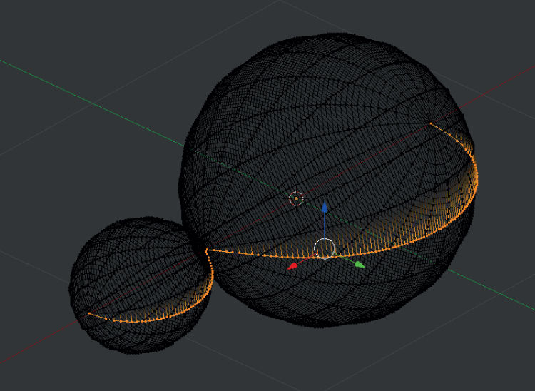
Figure 8.8. The zero-velocity curves can be mapped and then rotated in 3D using the spin tool in Mesh Edit mode.
The primary and secondary masses can be added at their respective positions with simple colored UV-spheres, as can the Lagrangian points, designated as small tetrahedrons (figure ).
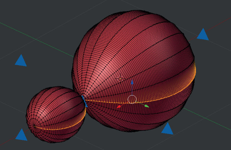
Figure 8.9. The Roche lobes can be rendered transparent via the Properties panel Materials tab.
8.5 Geophysics: planetary surface mapping
Blender is well suited for creating 3D surfaces from mapping data. In this project we will use topographic maps from the Mars MOLA Digital Terrain Topographic Maps to generate a 3D surface map []. This project introduces the following concepts:
- Importing an image as a plane.
- Using a displacement modifier.
- Mapping an image to a UV-plane.
- Using both a topographic map and color basemap imaging to layer textures.
The data are obtained from the USGS PDS Imaging Node. The two images each have a size and resolution of 1000 × 1000 pixels at 1.32 kilometers per pixel. The topographic map will be used for the relative heights between points on the surface for the Blender mesh object. The Mars basecolor map will be used as a texture layer.
First we will activate a new feature under File → User Preferences → AddOns. Click the check box for ‘Import Images as Planes’ and then ‘Save User Settings’. This will allow us to to image a topographic map directly as a mesh plane object.
The images need to be grayscale topographic maps and not shaded relief maps.
- Choose File → Import → Images as planes and select the topographic map file.
- Press the TAB key to enter Edit mode.
- Press the W key and select ‘Subdivide’. If a mesh division is less than the number of pixels in the image, the resulting mesh will be averaged. This is acceptable for quick look visualizations, but can be performed at full resolution in the final rendering.
- In the Properties panel select Modifiers → Displace. Select the texture to be the topographic map file. Set the strength (a convenience scaling factor) to 0.05. Set the texture coordinates to ‘UV’ (figure ).
- In the Properties panel select the Materials tab. Set the diffuse and spectral intensity to 0.0 and the shading emission to 1.0.
- In the Properties panel select the Textures tab. Add two textures—one for the displacement from the topographic map and one for the surface imaging. Their types need to be set to ‘Image or Movie’ and the coordinates to ‘UV’. For the surface imaging the diffuse influence should be set to ‘Color: 1.0’ and for the topographic map ‘Intensity: 1.0’. These settings are described in figure .
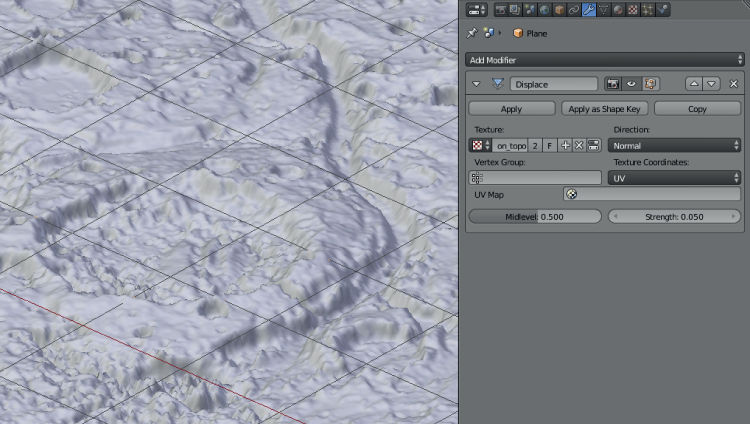
Figure 8.10. Setting up the displacement modifier to load the Martian topographic map into a mesh object.
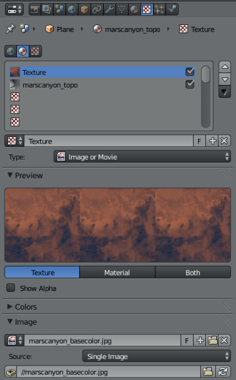
Figure 8.11. Terrain texture setting for Martian mapping.
The final composite as viewed normal to the plane is shown in figure .
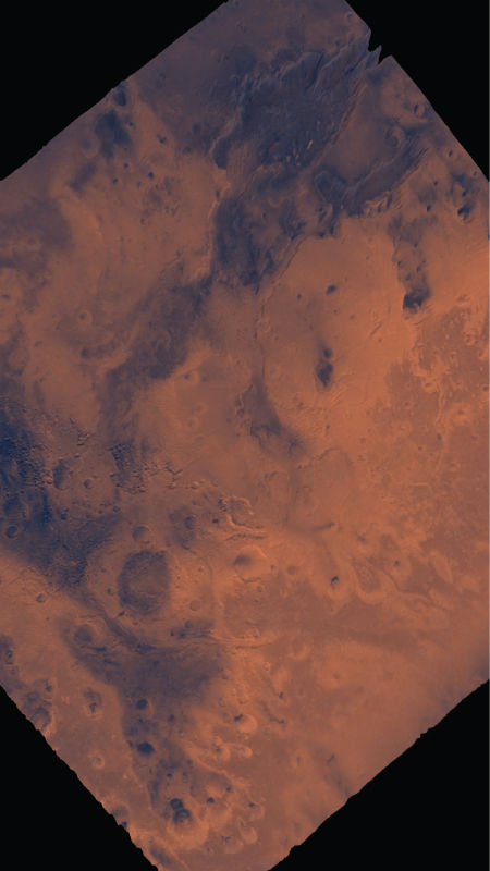
Figure 8.12. Mars terrain composite generated from a map displacement modifer and texture layer.
8.6 Volumetric rendering and data cubes
Data cubes are datasets composed of cross sections in a given phase space that are best viewed as rendered transparent volumes []. These kinds of data have applications in biology, medicine and astrophysics. CAT scan data provide slices of a scanned object with each element being a volumetric pixel (voxel). Data from radio telescopes that consist of right ascension and declination (positions on the celestial sphere) and frequency can be used to show the rotation of a galaxy or chemical species at millimeter wavelengths [].
In this application we utilize the following Blender functions:
- Loading cross section slices into Blender.
- Adding the data as a voxel ‘texture’.
- Setting the material and texture properties to render a volume.
For this example we will use CAT scan data of a human head that is easy to download and illustrates a simple example of volumetric rendering. Other excellent examples from radio astronomy and the NRAO radio telescope facilities can be found on-line as well.
- Begin with the default file that loads on Blender start-up.
- Right-click to select the default cube object. This will act as the data container.
- Scale the data container to match the data cube dimensions in the Transform dialog on the right-hand side of the GUI.
- Click on the Materials tab on the far right-hand side of the Properties panel.
- Click the ‘+’ button to add a new material. Select ‘Volume’ as the material type.
- The graphic densities have been set in the accompanying blend file. For different data these will have to be scaled appropriately by the user.
- Change the graphic density to 0.0 and density scale to 2.0.
- Under ‘Shading’ set the emission to 0.0 and scattering to 1.4.
The material type has been set and now the image slices can be applied to the texture for the mesh.
- Click the Textures tab on the Properties panel.
- Click the ‘+ New’ button to create a new texture.
- From the Type drop-down box choose ‘Voxel Data’.
- Check the ‘Ramp’ box and set the far right ramp color to that of your choosing. We will use a greyscale color for this example.
- Under the ‘Voxel Data’ section, open the first file in the image sequence.
- Change the ‘File Format’ and ‘Source’ to ‘Image Sequence’.
- Under ‘Mapping’ change the projection to ‘Cube’.
- Under ‘Influence’ select ‘Density’, ‘Emission’ and ‘Emission Color’ and set their values to 1.0 (figure ).
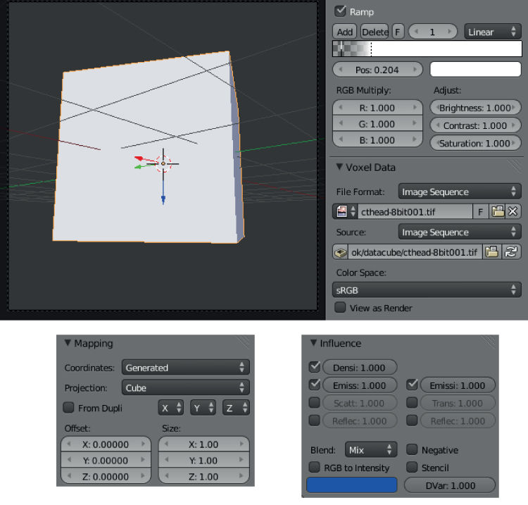
Figure 8.13. Set-up configuration for rendering a data cube.
Several views of the data cube are shown in figure . The procedure outlined here can be applied to any kind of 3D dataset that requires volume rendering for viewing []. A data cube from radio telescope observations is shown in figure [].
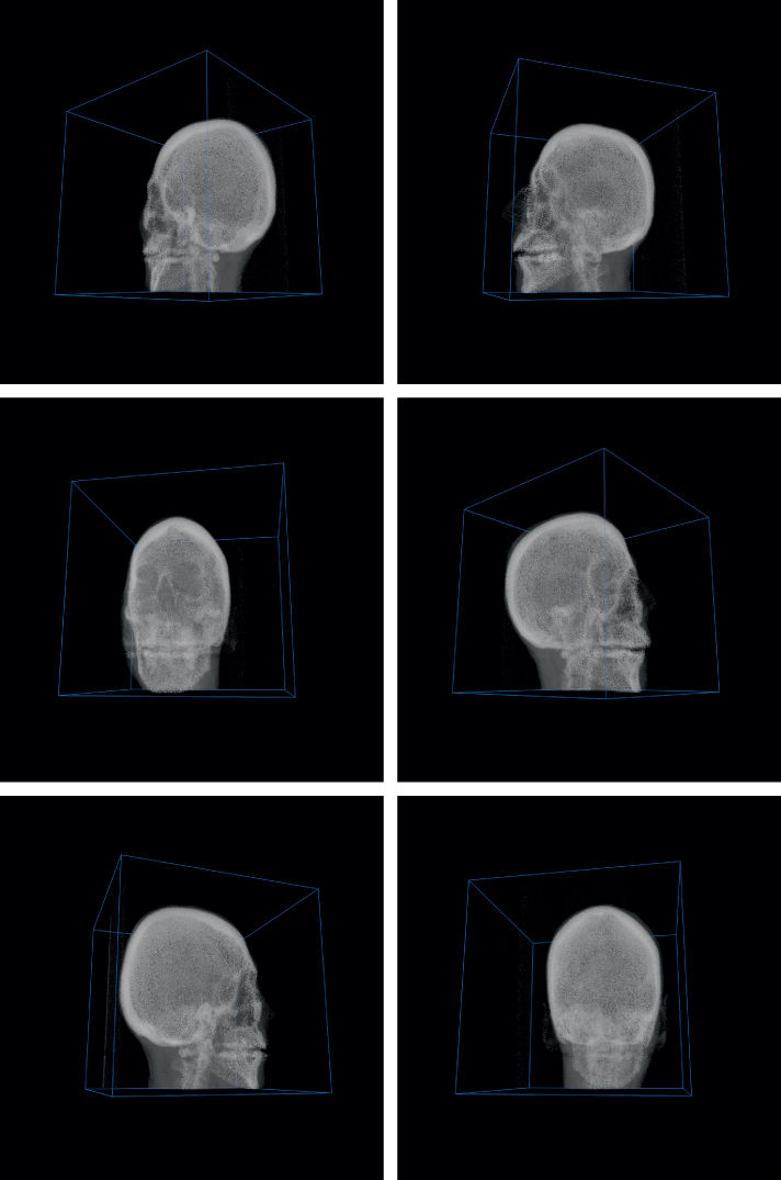
Figure 8.14. Rotating the volume rendering of a data cube.
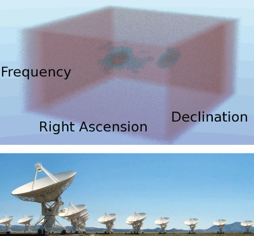
Figure 8.15. 3D rendering of a galaxy data cube obtained with observations from the National Radio Astronomy Observatory Very Large Array in New Mexico, USA.
8.7 Physics module and rigid body dynamics
The Blender physics module allows a user to use the built-in differential equation solver to add fields to a visualization scene and create physics demonstrations. Simple projectile motion, charged particles interacting with magnetic fields and simple harmonic motion are all possible with this module. The fields available to the user are shown in figure . In this project we will use the following concepts.
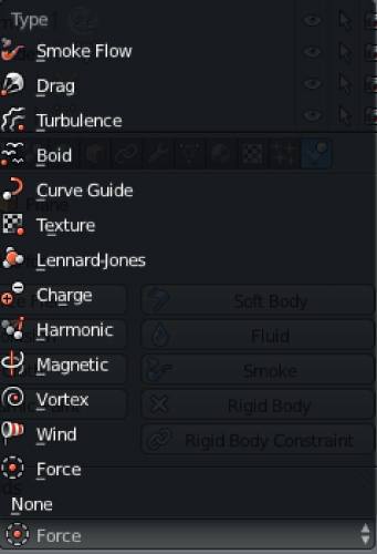
Figure 8.16. Fields available to the user with the Blender physics module. Mesh objects can be set to react to the physical constraints that occur because of a given field.
- Activate the Physics property tab.
- Set plane meshes as passive rigid bodies.
- Scale the simulation units to SI.
- Set time steps and compute the mesh positions (known as a bake) before running the animation to improve efficiency.
This example will combine a number of Blender physics module items and demonstrate their properties.
- Begin by Add → Mesh → Plane and scale the object with the S key.
- Choose the Physics module on the Properties panel (figure ).
- Select ‘Rigid Body’ and set the type to ‘Passive’.
- A ball (Add → Mesh → UV Sphere) should be added at a location Z = 1.0 above the plane.
- Choose the Physics module, select ‘Rigid Body’, and set the type to ‘Active’.
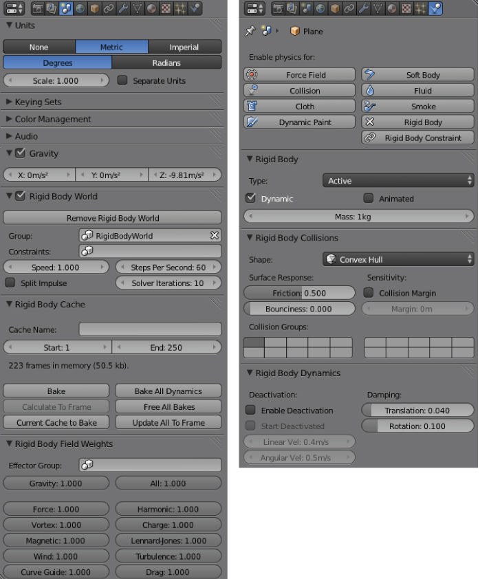
Figure 8.17. The Physics menu allows for the addition of fields to a visualization scene. These particular menus show the configuration for a fixed passive surface with rigidity and elasticity values. The acceleration due to gravity on Earth is set to the SI value of 9.8 m s−2, and the differential equation solver is set to 60 steps per second under the Scene menu.
Hitting the play button on the animation time line will compute the position of the ball with a = 9.8 m s−2 and no drag. The plane is passive and fixed, and therefore the ball simply stops. The ‘Surface Response’ for both the ball and the surface can be modified from a range of zero to one. With a maximum value of 1.0 for both objects the collision will be elastic with no energy dissipation—the ball will simply keep bouncing throughout the animation repeatedly. We will now create projectile motion by giving the ball an X-component to its initial velocity.
- Set the ‘Bounciness’ level to 0.5 for the sphere and 1.0 for the fixed plane.
- Add a second plane and rotate it with keys R–Y–90. Set the Physics module to ‘Rigid Body’ and ‘Passive’ just like the first plane. In addition, check the ‘Animation’ box.
- Keyframe the X-location for the first and tenth frame. Due to the rigid body dynamics we have now set up, the plane will give the ball an X velocity.
- Set the ‘Friction’ value for the fixed ground plane to 0.0.
Pressing the play button one more time from the beginning will now show the ball exhibiting projectile motion.
We will use the mesh screw tool and multiple spheres to finish the rigid body dynamics example.
- Add → Mesh → Circle to create the start of a rigid body tube.
- Enter Mesh Edit mode with the TAB key and add a rotation vector as shown in figure .
- Activate the screw tool on the left-hand side of the GUI and set the number of steps to 48.
- A corkscrew tube will be created. Press the TAB key again to enter Object mode and select the Physics Module tab. Set the ‘Rigid Body’ object to be ‘Passive’ with a ‘Mesh’ collision shape instead of the default ‘Convex Hull’. This will allow the ball to roll inside the tube.
- Move the corkscrew relative to the plane mesh object such that the lower opening will allow the ball to roll out onto the plane.
- Change the sphere object’s collision shape to ‘Sphere’ and place it at the top of the corkscrew tube.
- Duplicate the sphere with SHIFT–D and place the new objects on the flat plane (figure ).
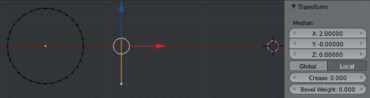
Figure 8.18. The initial set-up for a rigid body simulation. This example from the Mesh Edit window shows the set-up for a circle and rotation vector. The screw tool will be used to rotate the vertices about an incline to create a corkscrew tube shape. This shape will have a mesh collision shape in the Physics module such that another sphere can roll inside the tube.
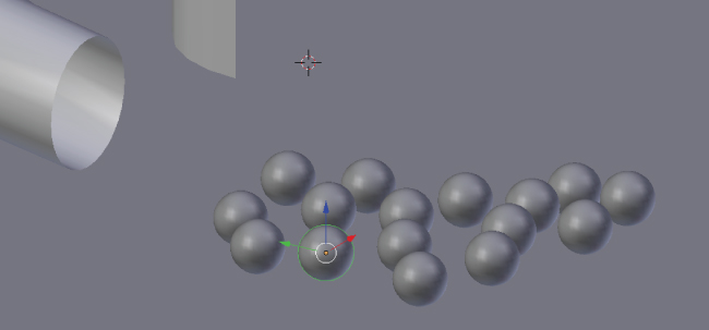
Figure 8.19. UV-sphere mesh objects with a spherical collision shape set in the Physics module are duplicated with SHIFT–D. The objects and properties are duplicated and set up for a collision.
The simple elements for our rigid body dynamics simulation are in place. The last step will be to bake the simulation elements and compute all the positions. As depicted in figure , press the ‘Free All Bakes’ button followed by ‘Bake’. Press the play button on the animation time line to view the simulation (figure ).
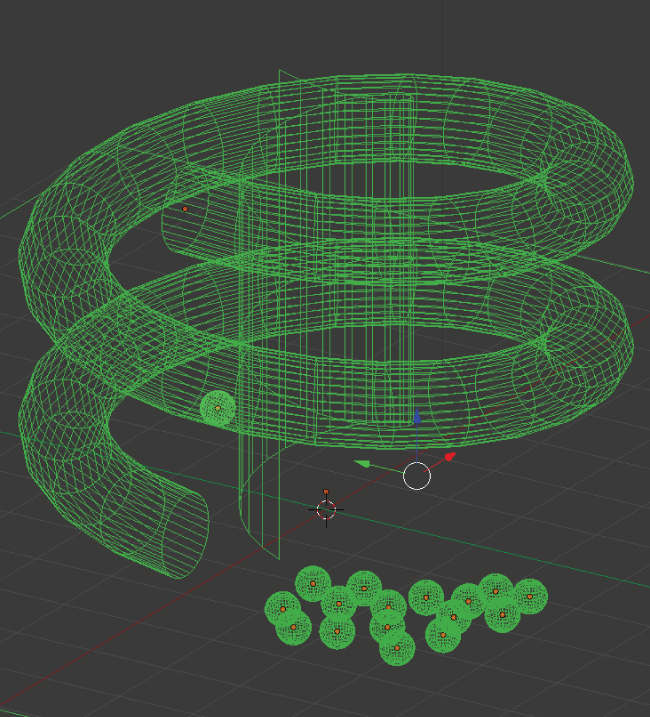
Figure 8.20. The physics menu allows for the addition of fields to a visualization scene. These particular menus show the configuration for a fixed passive surface with rigidity and elasticity values. The acceleration due to gravity on is set to the SI value of 9.8 m s−2 and the differential equation solver is set to 60 steps per second under the Scene menu.
For longer simulations, baking will take significantly longer depending on factors like the number of vertices and fields in the simulation. However, by baking in the dynamics and performing the computation a priori, the rendering time will be significantly decreased.
Bibliography
[1] Perryman M A C et al 1997 The HIPPARCOS catalogue Astron. Astrophys. 323 L49–52
[2] Springel V 2005 The cosmological simulation code GADGET-2 Mon. Not. R. Astron. Soc.
[3] Jackson J D 1999 Classical Electrodynamics 3rd edn (New York: Wiley)
[4] Murray C D and Dermott S F 1998 Solar System Dynamics (Cambridge: Cambridge University Press)
[5] Christensen P R et al Mars global surveyor thermal emission spectrometer experiment: investigation description and surface science results J. Geophys. Res.
[6] Levoy M 1988 Volume rendering: display of surfaces from volume data Comput. Graphics Appl.
[7] Hassan A H, Fluke C J and Barnes D G 2011 Interactive visualization of the largest radioastronomy cubes New Astron.
[8] Kent B R 2013 Visualizing astronomical data with Blender Publ. Astron. Soc. Pac.
[9] Walter F et al 2008 THINGS: The H I Nearby Galaxy Survey Astron. J.
For excellent research on this topic using simulations of cataclysmic variable stars, visit .
Images and data available from .

